To describe the material behavior of polymer blends, the same material properties must be investigated and characterized as for neat polymers.

If, in addition to general calculations, the morphology development of a polymer blend is to be simulated, the interfacial energetic properties of the polymer combination must also be analyzed and described.

The interfacial tension can be determined experimentally using various methods, including:

• Breaking Thread,
• Pendant Drop, and
• Spinning Drop.

The Breaking Thread method is based on the theoretical description of the breakup of a liquid Newtonian filament in a Newtonian matrix. However, this method is limited to multiphase systems in which the melting temperature of the dispersed phase is higher than that of the matrix. Furthermore, the zero-shear viscosity $η_0$ (viscosity $η$ at $\dot γ → 0$) of the matrix should not exceed 40 kPas. A schematic of the experimental setup used for the measurements is shown in the next figure. During the entire test, the heating stage is purged with nitrogen. Before the measurement starts, the system is conditioned in the heating stage at 220 °C for approximately 10 minutes in order to minimize retardation effects during melting. Subsequently, the system is heated up to the desired test temperature. As soon as the filament is completely molten, capillary waves form at its interface with the matrix. The entire process is recorded using a CCD camera.

These sinusoidal capillary waves or filament neckings are captured at large time intervals and evaluated by computer analysis.

PLATZHALTER ABBILDUNG 111: Versuchsaufbau zur Erfassung und Auswertung von dispersen Fadenzerfallsprozessen mit einem Heiztisch zur Bestimmung der Grenzflächenspannung

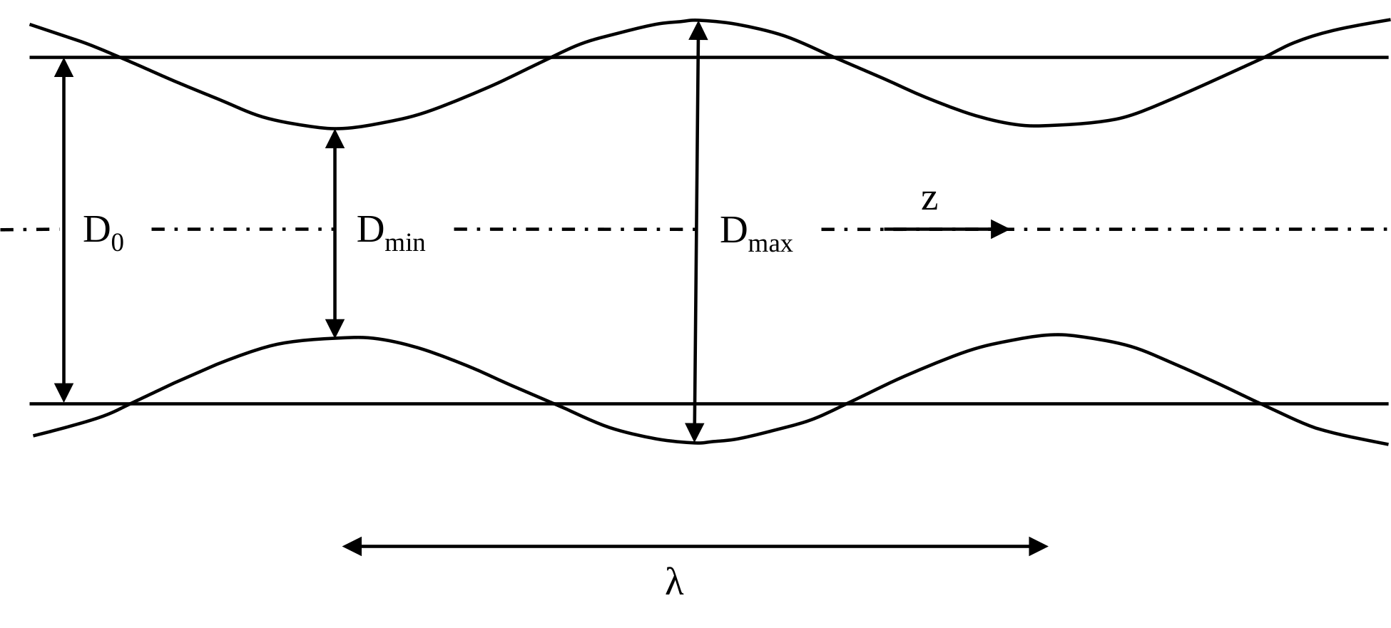
For the filament, the initial diameter $D_0$, the wavelength $λ$, as well as the maximum and minimum filament diameters $D_{max}$ and $D_{min}$ are measured. The following figure shows the characteristic form of such a capillary wave with its relevant dimensions for theoretical consideration.

The interfacial tension $γ_{12}$ is then a function of the amplitude growth rate $q$, the dimensionless growth rate $Ω$, the matrix viscosity $η_c$, and the initial filament diameter $D_0$, and can be expressed as:

$$γ_{12} = \frac {q \cdot η_c \cdot D_0}{Ω(p,X)}$$

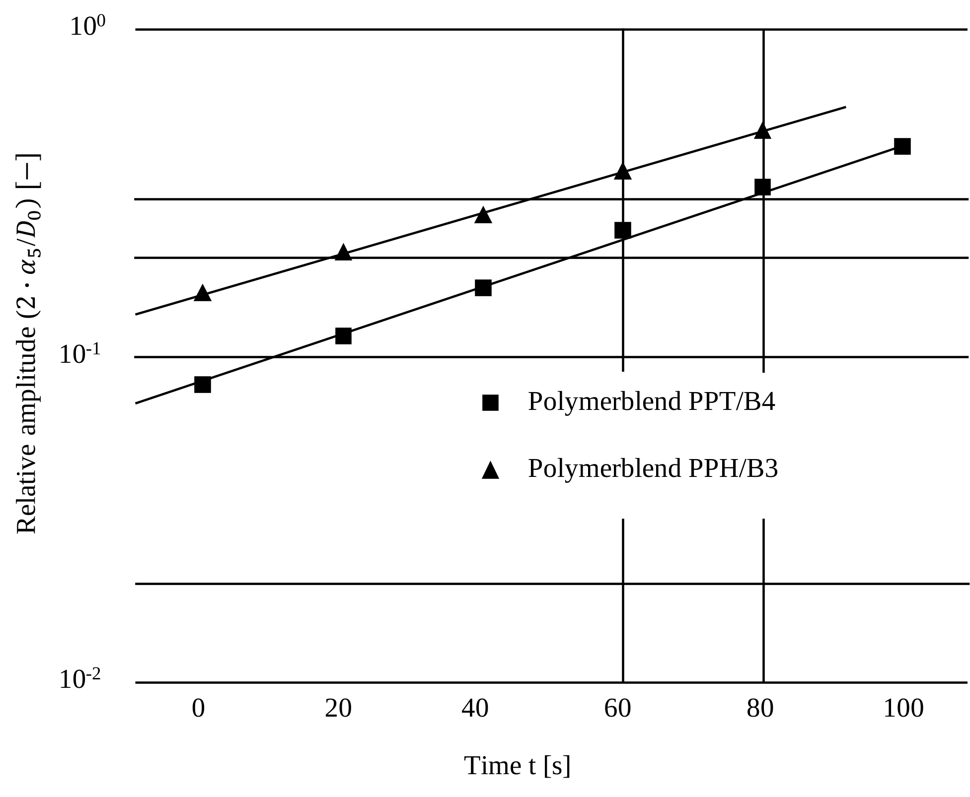
The amplitude growth rate $q$ can be determined from the slope $S$ of the relative amplitude $log (2 \cdot α_s / D_0)$ plotted against time $t$:

$$q = S \cdot ln 10$$

For the oscillation amplitude, the following relation applies:

$$α_s = \frac {D_{max} - D_{min}}{4}$$

For calculating the interfacial tension $γ_{12}$ in this work, the dimensionless growth rate $Ω(p,X)$ is used. The viscosity ratio is defined as:

$$p = \frac {η_d}{η_c}$$

and the wavenumber, determined experimentally, is defined as:

$$X= \frac {π \cdot D_0}{λ}$$

The next figure shows the behavior of the dimensionless growth rate $Ω$ as a function of the viscosity ratio $p$ and the wavenumber $X$. The solid line indicates the maxima of the dimensionless growth rate $Ω_m$.

If the determined $γ_{12}$ values are plotted against different temperatures $T$, the data points above the crystalline melting temperature $T_K$ (for semi-crystalline polymer pairs) or glass transition temperature $T_G$ (for amorphous polymer pairs) can be approximated by a linear function of the form:

$$γ_{12} (T) = γ_{12.0} - γ_{12.m} \cdot T$$

PLATZHALTER ABBILDUNG 114: Dimensionslose Wachstumsrate als Funktion der Wellenzahl X und des Viskositätsverhältnisses p

Here, $γ_{12.0}$ represents the intercept of the approximation function with the ordinate, while $γ_{12.m}$ corresponds to the slope of this function. The following figure illustrates the typical course of interfacial tension $γ_{12}$ as a function of temperature $T$ for a polypropylene (PP) / polyamide (PA6) blend.

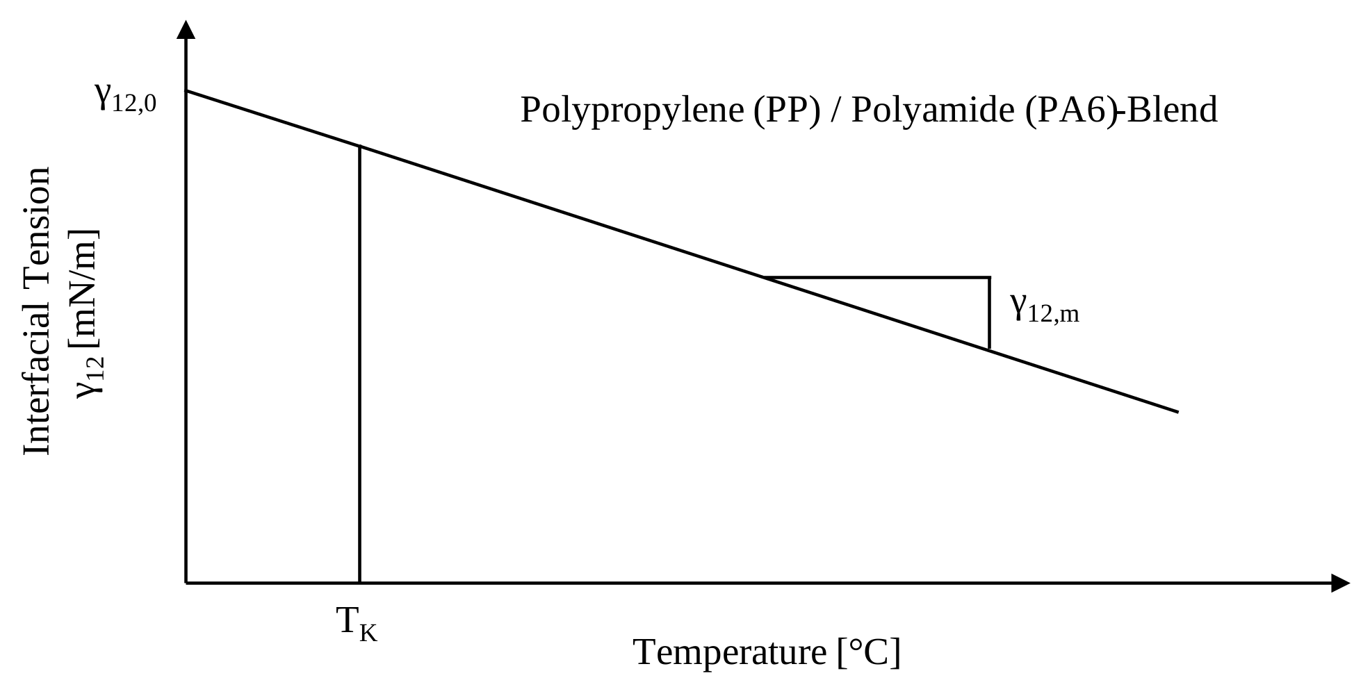
In the literature, the slope of this straight line is typically approximated by $γ_{12.m} = 0.01 , mN/m°C$. In practice, however, this value varies from one polymer pair to another. Therefore, to establish the approximation function, only two measurements of the interfacial tension $γ_{12}$ at two different temperatures $T$ are required. This allows the Breaking Thread Method to provide a rapid determination of interfacial tension $γ_{12}$ above the melting temperature $T_K$ with minimal experimental effort.

The pendant Drop method is the most versatile and reliable technique for measuring both surface and interfacial tensions of polymers. On the one hand, this is because equilibrium between the polymer phases is usually achieved more quickly compared to other methods, and on the other hand, because measurements can also be performed in an inert atmosphere.

The method is based on the optical measurement of the shape of a liquid or molten drop that is in hydrostatic equilibrium with the surrounding phase. The droplet profile is compared with the theoretically predictable droplet shape, which can be calculated based on the Gauss-Laplace equation. The interfacial (or surface) tension is then obtained as:

$$γ_{12} = g \cdot Δρ \cdot d_1^2 \cdot \frac{1}{H}$$

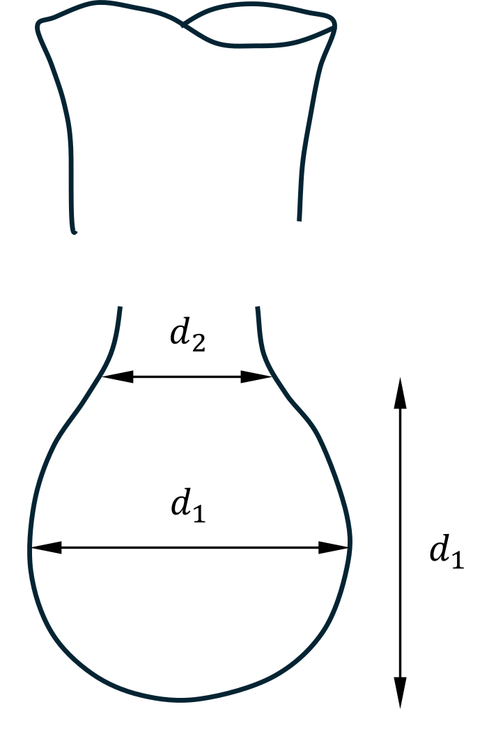
where $g$ is gravitational acceleration, $Δρ$ is the density difference between the polymer phases, and $\frac {1}{H}$ is a correction factor, whose value depends on the shape factor $S$:

$$S= \frac {d_2}{d_1}$$

Here, $d_1$ is the maximum droplet diameter and $d_2$ the droplet diameter at a distance $d_1$ from the apex. Values of the correction factor $\frac {1}{H}$ can be obtained numerically from tabulated data using the following equations (piecewise in dependence on $S$):

$$\frac {1}{H} = (\frac {0,32720}{S^{2,56651}}) - 0,97553 \cdot S^2 + 0,84059 \cdot S - 0,18069$$

for $0.401 ≤ S ≤ 0.46$,

$$\frac {1}{H} = (\frac {0,31968}{S^{2,39725}}) - 0,46898\cdot S^2 + 0,50059\cdot S - 0,13261$$

for $0.46 ≤ S ≤ 0.59$,

$$\frac {1}{H} = (\frac {0,31522}{S^{2,62435}}) - 0,11714\cdot S^2 + 0,15756\cdot S - 0,05285$$

for $0.59 ≤ S ≤ 0.68$,

$$\frac {1}{H} = (\frac {0,31345}{S^{2,61267}}) - 0,09155\cdot S^2 + 0,14701\cdot S - 0,05877$$

for $0.68 ≤ S ≤ 0.90$,

$$\frac {1}{H} = (\frac {0,30715}{S^{2,84636}}) - 0,69116 \cdot S^3 + 1,08315\cdot S^2 - 0,18341\cdot S - 0,20970$$

for $0.90 ≤ S ≤ 1.00$.

Thus, the interfacial or surface tension can be calculated from the two droplet diameters and the melt densities. However, it must be ensured that the molten droplet is in equilibrium with its surrounding phase. For low-viscosity Newtonian fluids, this is usually the case immediately, while for highly viscous or viscoelastic melts, equilibrium can take several hours.

Apart from the optical requirements, this method is relatively simple in terms of apparatus, but in practice it requires significant skill to generate droplets suitable for evaluation. Additionally, various experimental conditions must be considered. Since density differences $Δρ$ enter the calculation, reliable melt density data are required. However, for polymers, such data are only sparsely available at arbitrary temperatures and thus must be determined experimentally, which introduces error. Further, practical limitations exist: for interfacial tension measurements, the droplet must be formed in the continuous melt phase of a second polymer. Suitable material combinations must therefore meet the conditions of immiscibility, sufficiently low viscosity of the continuous phase, and transparency to enable optical recording. Moreover, gas release or decomposition during melting may cause bubble formation, which distorts the droplet shape and leads to unrealistic results.

The principle of the spinning drop method is also based on the measurement of droplet shape, but here the contour develops under the influence of centrifugal force. When a cylindrical capillary containing a droplet and a denser liquid is rotated around its longitudinal axis at constant high speeds (2000–8000 rpm), the droplet assumes a cylindrical shape with rounded ends.

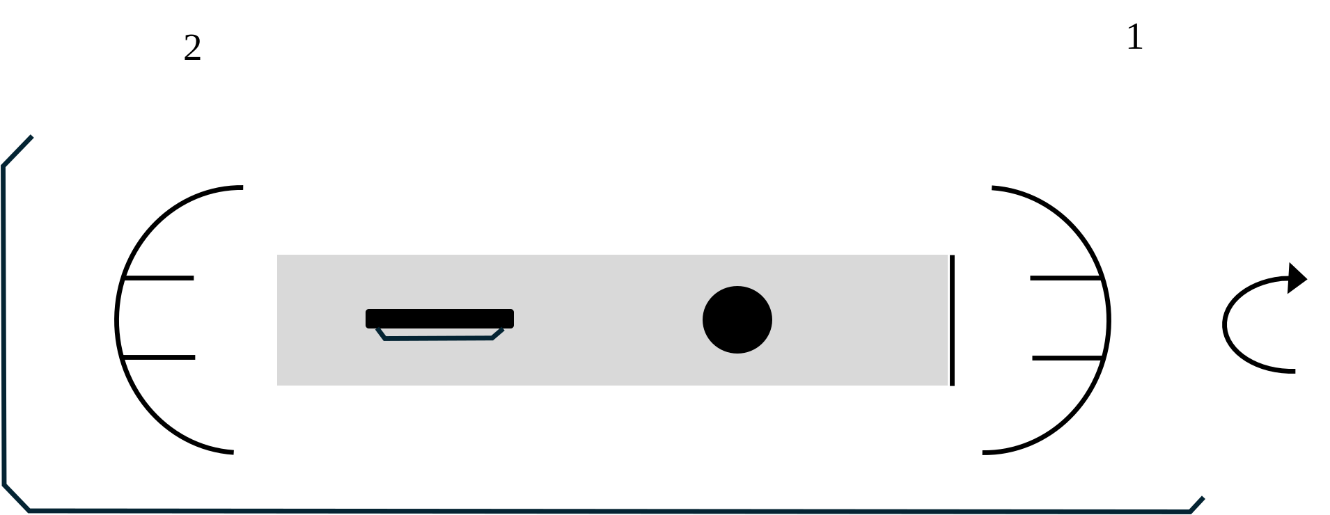
The droplet profile is governed by interfacial (or surface) tension, density difference, and centrifugal force. Since gravitational effects can be neglected, the interfacial tension can be expressed as:

$$γ_{12} = \frac {Δρ \cdot ω^2}{4 \cdot Q}$$

where $ω$ is the angular velocity of the capillary and $Q$ is a constant defined by:

$$L_0 = \frac{(\frac{4}{3}) \cdot (Q \cdot R^3 +1)}{(Q \cdot R^3)^\frac{1}{3}}$$

Here, $L_0$ is the equilibrium length of the spinning droplet and $R$ is the droplet radius.

This method has proven particularly suitable for systems with extremely low interfacial tensions, with modern instrumentation enabling measurements down to $10^{-5}$–$10^{-6}$ mN/m. Moreover, this principle ensures that the interface is not disturbed by foreign objects, and demixing phenomena as well as interfacial phase formation can be observed. A disadvantage of this method is the slow attainment of equilibrium. For example, in measurements with fluids of intermediate viscosity (300–500 Pas), equilibrium was only reached after more than three hours at 6100 rpm.