The rheological as well as the thermodynamic parameters of two-component systems (e.g., solidification and melting enthalpies of polymer blends) generally cannot be determined with sufficient accuracy by a simple linear averaging of the data of the base components. For simulations with REX / PSI / SIGMA, this means that, prior to the actual simulation runs, complete material data for the polymer blends should ideally be determined experimentally. However, this requires a considerable amount of measurements even before the simulation process itself can be carried out. If, on the other hand, only the material data of the individual components are available, the material data of the blends are calculated within REX / PSI / SIGMA from the component data as follows.

For calculating the viscosity of two-phase polymer blends, the literature provides a range of mixing rules that vary in complexity depending on the required level of accuracy—from simpler approaches to more mathematically elaborate ones. In the simulation software packages REX / PSI / SIGMA, the following general mixing rules are applied:

first, the simplest and most widely used logarithmic mixing rule according to Arrhenius:

$$log η_{MIX} = w_1 \cdot log η_1 + w_2 \cdot log η_2$$

and second, the mixing rule proposed by Mantford:

$$(η_{MIX})^{1/3,4} = w_1 \cdot η_1^{1/3,4} + w_2 \cdot η_2^{1/3,4}$$

The determination of the blend viscosity from the viscosities of the individual components $η_i$ and their weight fractions $W_i$ using REX / PSI / SIGMA is illustrated in the following figure.

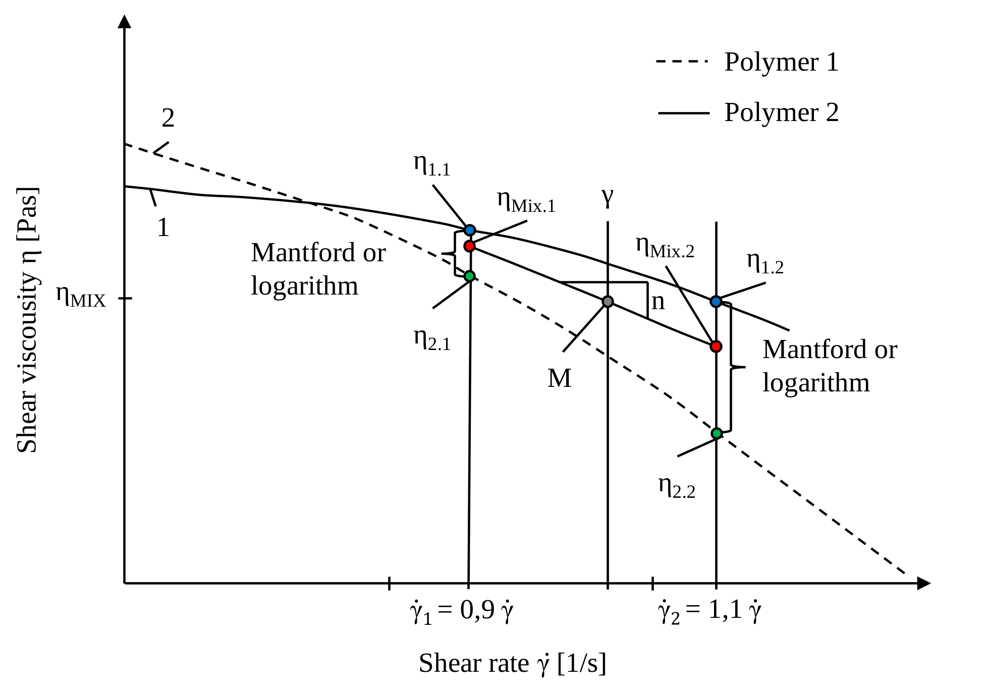
To calculate the viscosity $η_{MIX}$ at a given shear rate $\dot γ$ for a polymer blend, the blend viscosities $η_{MIX1}$ and $η_{MIX2}$ are first determined for the defined shear rates $\dot γ_1 = 0.9 \cdot \dot γ$ and $\dot γ_2 = 1.1 \cdot \dot γ$. For the Mantford approach, the following applies:

$$(η_{MIX1})^{1/3,4} = w_1 \cdot η_1.1^{1/3,4} + w_2 \cdot η_2.1^{1/3,4}$$ $$(η_{MIX2})^{1/3,4} = w_1 \cdot η_1.2^{1/3,4} + w_2 \cdot η_2.2^{1/3,4}$$

Analogously, the logarithmic mixing rule (Arrhenius) is given by:

$$log η_{MIX1} = w_1 \cdot log η_1.1 + w_2 \cdot log η_2.1$$ $$log η_{MIX2} = w_1 \cdot log η_1.2 + w_2 \cdot log η_2.2$$

If these quantities are known, the flow behavior index $n$ and the consistency $K$ of the approximated blend segment between $\dot γ_1 = \dot γ_{MIX1}$ and $\dot γ_2 = \dot γ_{MIX2}$ can be determined as follows:

$$n = 1 + \frac{log(\frac{η_{MIX1}}{η_{MIX2}})}{log(\frac{\dotγ_{MIX1}}{\dotγ_{MIX2}})}$$

$$K = \frac{η_{MIX1}}{\dotγ_{MIX1}^{n-1}}$$

The desired viscosity $η_{MIX}$ is finally obtained by:

$$η_{MIX} = K \cdot \dotγ_{MIX}^{n-1}$$

If the dispersed phase is present in solid or highly viscous form, the system can be regarded as a filled polymer. For simulation purposes, in the case of a filled polymer the base polymer and its particle diameter must first be defined. The filler is then specified. This requires a range of material data: the particle diameter $d$, the mass fraction $w$, the solid density $ρ$, the bulk density $ρ_s$, the thermal conductivity of the solid $λ_0$, and the specific heat capacity $c_0$. Similar to polymer blends, two mixing equations are also available for filled polymers. The first is the simple approach according to Einstein:

$$η_{MIX} = η_1 \cdot (1 + 2,5 \cdot Φ_2)$$

and finally, the approach according to Hashin:

$$η_{MIX} = η_1 \cdot [1+2 \cdot \frac{Φ_2}{1-Φ_2}]$$

In these equations, $η_1$ denotes the viscosity of the base polymer, and $Φ_2$ the volume fraction of the added component.

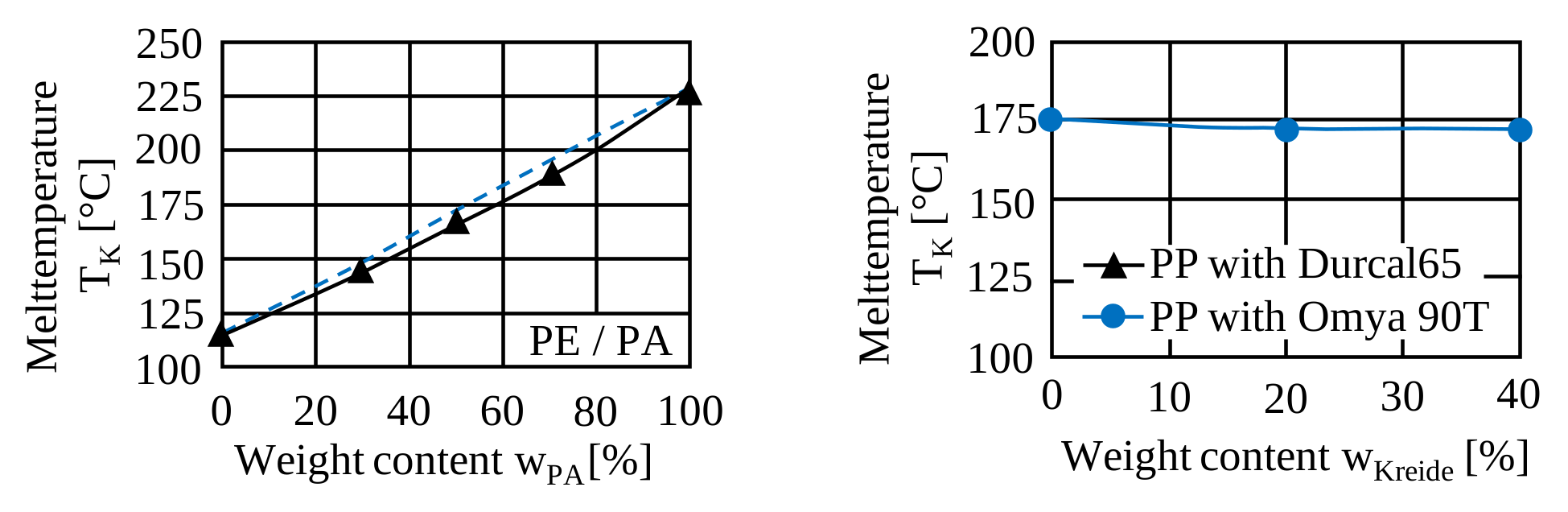
Experimentally determined crystalline melting temperatures, both for polymer blends and for filled systems (compounds), are shown in the following figure. For polymer blends, the crystalline melting temperature $T_{K.MIX}$ is calculated in REX / PSI / SIGMA from the weight fractions $w_i$ and the crystalline melting temperatures $T_{Ki}$ as follows:

$$T_{K.MIX} = w_1 \cdot T_{K.1} + w_2 \cdot T_{K.2}$$

whereas for compounds, the following applies:

$$T_{K.MIX} = T_{K.1}$$

The crystalline melting temperature $T_{K.MIX}$ of a filled polymer (compound) is therefore assumed to be equal to the crystalline melting temperature $T_{K1}$ of the base polymer.

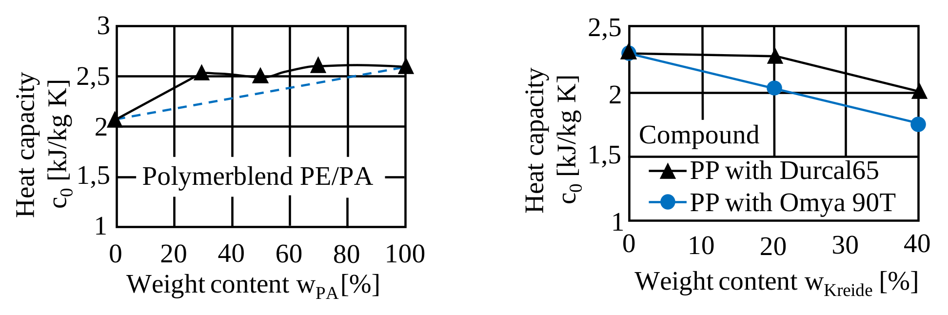
To describe the specific heat capacity $c$ of multicomponent systems, a uniform mixing rule is applied for both polymer blends and filled systems. For the specific heat capacity of the mixture $c_{MIX}$, the following applies:

$$c_{MIX} = w_1 \cdot c_1 + w_2 \cdot c_2$$

where $w_i$ are the weight fractions and $c_i$ the specific heat capacities of the individual or added components.

The specific heat capacity $c_{0.MIX}$ of the mixture is therefore given by:

$$c_{0.MIX} = w_1 \cdot c_{0.1} + w_2 \cdot c_{0.2}$$

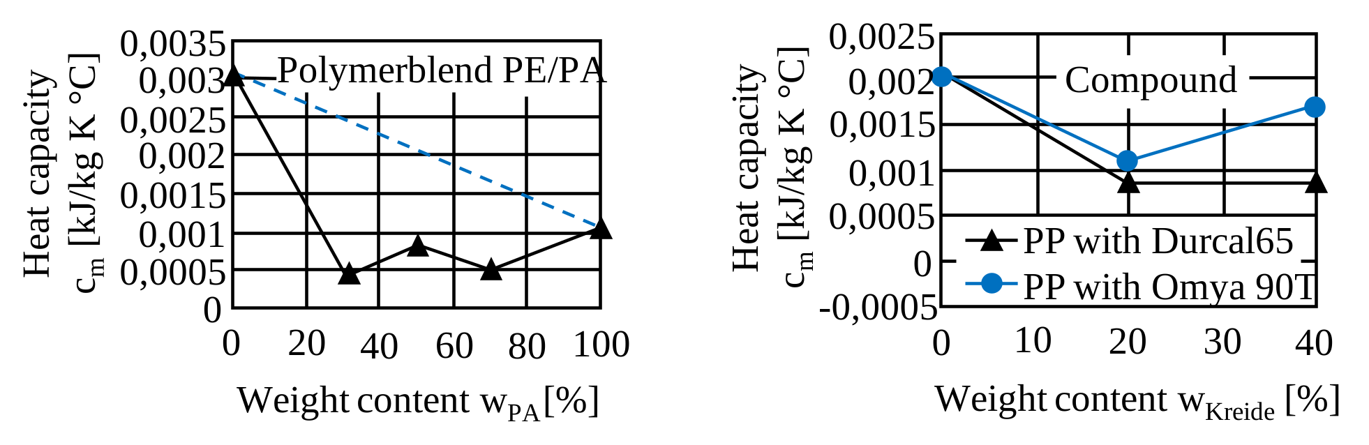
The following figure shows the course of the specific heat capacity $c_0$ for polymer blends and filled systems. The slope of the heat capacity curve, $c_{m.MIX}$, for the mixture is determined for both systems analogously according to the following equation:

$$c_{m.MIX} = w_1 \cdot c_{m.1} + w_2 \cdot c_{m.2}$$

The relationship between the specific heat capacity $c_m$ and the weight fractions for polymer blends and filled systems is illustrated as an example:

The specific enthalpy is given by:

$$Δh = w_1 \cdot Δh_1 + w_2 \cdot Δh_2 = w_1 \cdot {(Δh_F + Δh_A)}_1 + w_2 \cdot {(Δh_F + Δh_A)}_2$$

Index 1 refers to polymer 1 and index 2 to polymer 2.

For describing the specific enthalpy $Δh$ of filled systems (compounds), the following approach is used:

$$Δh = w_1 \cdot {(Δh_F + Δh_A)}_1 + w_2 \cdot c_2 \cdot ΔT$$

Here, index 1 refers to the polymer, while index 2 denotes the filler.

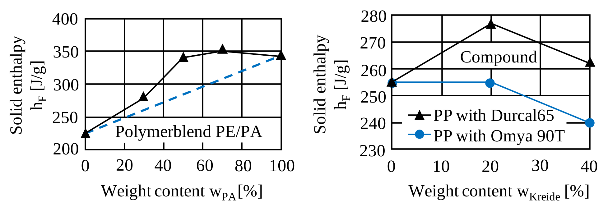
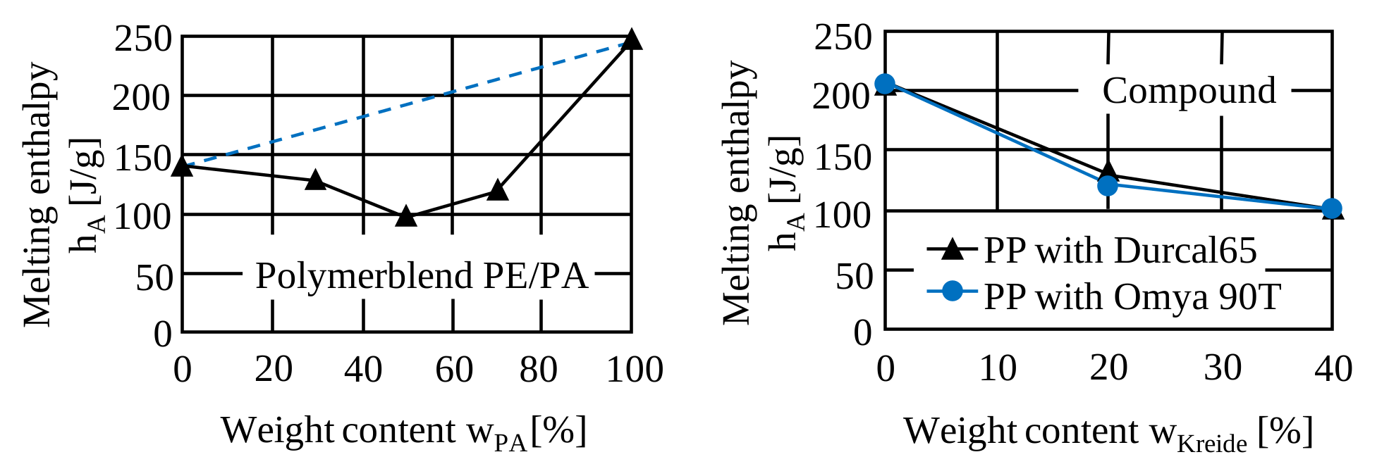
The solid enthalpy $Δh_F$ and melting enthalpy $Δh_A$ for polymer blends can be determined from the enthalpy values of the individual components as follows. For the solid enthalpy $Δh_{F.MIX}$ and melting enthalpy of the mixture $Δh_{A.MIX}$:

$$Δh_{F.MIX} = w_1 \cdot Δh_{F.1} + w_2 \cdot Δh_{F.2}$$

$$Δh_{A.MIX} = w_1 \cdot Δh_{A.1} + w_2 \cdot Δh_{A.2}$$

Analogously, for compounds (filled systems), the solid enthalpy $Δh_{F.MIX}$ and melting enthalpy $Δh_{A.MIX}$ of the mixture are calculated as follows:

$$Δh_{F.MIX} = w_1 \cdot Δh_{F.1}$$

$$Δh_{A.MIX} = w_1 \cdot Δh_{A.1} + w_2 \cdot c_2 \cdot ΔT$$

The following figures show, as examples, results from experimental investigations of the specific solid enthalpy $Δh_F$ and specific melting enthalpy $Δh_A$ of multicomponent systems.

In the simulation programs REX / PSI / SIGMA, the following equations are used to determine the thermal conductivity $λ_{MIX}$ of multicomponent systems from the values of the individual polymers ($w_i$, $λ_i$). For polymer blends:

$$λ_{MIX} = w_1 \cdot λ_1 + w_2 \cdot λ_2$$

For filled polymers (compounds), the following relationship is assumed for calculating the thermal conductivity:

$$λ_{MIX} = λ_2 \cdot \frac{λ_1 + 2 \cdot λ_2 - 2 \cdot Φ_1 \cdot (λ_2 - λ_1)}{λ_1 + 2 \cdot λ_2 + Φ_1 \cdot (λ_2-λ_1)}$$

While indices 1 and 2 correspond to the individual polymers 1 and 2 in polymer blends, for filled systems index 1 refers to the base polymer and index 2 to the added filler. For each component, the linear approximation is applied:

$$λ_i = λ_{0.i} + λ_{m.i} \cdot T$$

Here, $λ_{0.i}$ is the value of the linear approximation for the thermal conductivity of a component at $T = 0°C$, while $λ_{m.i}$ is the slope of the approximated thermal conductivity curve of the component above the melting temperature. For polymer blends, the thermal conductivity of the mixture $λ_{0.MIX}$ is:

$$λ_{0.MIX} = w_1 \cdot λ_{0.1} + w_2 \cdot λ_{0.2}$$

The slope of the mixture’s thermal conductivity function $λ_{m.MIX}$ is calculated as:

$$λ_{m.MIX} = w_1 \cdot λ_{m.1} + w_2 \cdot λ_{m.2}$$

For filled polymers (compounds), the following mixing equations are used to determine $λ_{0.MIX}$ and $λ_{m.MIX}$:

$$λ_{0.MIX} = λ_{0.2} \cdot \frac{λ_{0.1} + 2 \cdot λ_{0.2} -2 \cdot Φ_1 \cdot (λ_{0.2} - λ_{0.1})}{λ_{0.1} + 2 \cdot λ_{0.2} + Φ_1 \cdot (λ_{0.2} - λ_{0.1})}$$

and

$$λ_{m.MIX} = λ_{m.2} \cdot \frac{λ_{m.1} + 2 \cdot λ_{m.2} -2 \cdot Φ_1 \cdot (λ_{m.2} - λ_{m.1})}{λ_{m.1} + 2 \cdot λ_{m.2} + Φ_1 \cdot (λ_{m.2} - λ_{m.1})}$$

The calculation of the solid and melt density $ρ_{MIX}$ of polymer blends and compounds from the densities $ρ_i$ and weight fractions $w_i$ of the individual polymers or of the base polymer and filler follows the same equation:

$$\frac {1}{ρ_{MIX}} = \frac{w_1}{ρ_1} + \frac{w_2}{ρ_2}$$

The specific volume $v$ of polymer blends and compounds from the specific volumes $v_i$ and weight fractions $w_i$ of the individual polymers or of the base polymer and filler is calculated using:

$$v_{MIX} = w_1 \cdot v_1 + w_2 \cdot v_2$$

For polymer blends and filled polymers (compounds), the mixture values $v_{0.MIX}$ and $v_{m.MIX}$ are determined using:

$$v_{0.MIX} = w_1 \cdot v_{0.1} + w_2 \cdot v_{0.2}$$

and

$$v_{m.MIX} = w_1 \cdot v_{m.1} + w_2 \cdot v_{m.2}$$

To determine the bulk density $ρ_{S.MIX}$ of multicomponent systems such as polymer blends and compounds with granule diameters $d_1$ and $d_2$ (where $d_1 < d_2$) of the individual components or of the base polymer and filler, some considerations must first be made. The following figure illustrates the bulk density $ρ_{S.MIX}$ of a mixture composed of two different particle fractions.

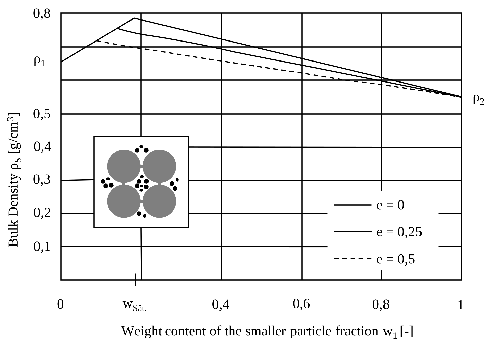
For both polymer blends and filled systems (compounds), the granule diameter of the smaller fraction is assumed to be much smaller than that of the larger fraction ($d_1 \ll d_2$). If the bulk density $ρ_{S.MIX}$ of a mixture composed of two different particle fractions is plotted against the weight fraction of the smaller fraction $w_1$, each curve exhibits a maximum at the saturation concentration $w_1 = w_{Sät}$, independent of the void fraction $e$. The saturation concentration is calculated as:

$$w_{Sät} = \frac {ρ_2 \cdot (1-p_∞) \cdot (1-e)}{ρ_1 + ρ_2 \cdot (1-p_∞) \cdot (1-e)}$$

with the maximum packing fraction for a cubic-close-packed arrangement of spheres:

$$p_∞ = \frac {V_{Kugel}}{V_{Gesamt}} = \frac {π}{3 \cdot √2} ≈ 0,74$$

Here, $V_{sphere}$ is the volume that the larger material component (Mat. 2) can maximally occupy relative to the total volume $V_{total}$. The void fraction that is too small for the smaller component (Mat. 1) to fit is set to $e = 0.25$. From this, the saturation bulk density (bulk density of the mixed region) is obtained:

$$ρ_{Sät} = ρ_1 + (1-ρ_∞) \cdot (1-e) \cdot ρ_2$$

To determine the bulk density $ρ_{S.MIX}$ of multicomponent systems in polymer blends and compounds with $d_1 < d_2$, three cases are distinguished. The procedure for the three calculation types is illustrated in the following figure. The subdivision criterion in all calculation types is the ratio of the particle diameters ($d_1 / d_2$). Initially, only two calculation approaches are used ($d_1 < 0.25 \cdot d_2$ or $d_1 > 0.75 \cdot d_2$), while the third calculation approach is obtained by linear averaging of the other two in the transition range ($0.25 \cdot d_2 < d_1 < 0.75 \cdot d_2$).

• if $w_1 < w_{Sät}$

$$\rho_{Mix} = \left(1 - \frac{w_1}{w_{Sät}}\right)\rho_1 + \frac{w_1}{w_{Sät}} \rho_{Sät}$$

• if $w_1 \geq w_{Sät}$

$$\rho_{Mix} = \left(1 - \frac{1 - w_1}{1 - w_{Sät}}\right)\rho_2 + \frac{1 - w_1}{1 - w_{Sät}} \rho_{Sät}$$

$$\frac{1}{\rho_{Mix}} = \frac{w_1}{\rho_1} + \frac{w_2}{\rho_2}$$

$$\rho_{Mix} = \frac{(\rho_{Mix I} + \rho_{Mix II})}{2}$$

Here, $\rho_{Mix}$ is obtained by linear averaging of Calculation Types I and II.