Dies ist eine alte Version des Dokuments!
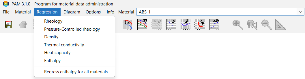
Menu Regression
Evaluation of the Measurements
The measurement data entered can be evaluated using various predefined regression functions. The data determined in this way is then automatically transferred to the data record for the corresponding material. Measurement series can only be evaluated if they have been assigned a specific measurement type (rheology, density, specific heat capacity, etc.). No evaluation is possible for Free measurement types.
The regression can be performed either in the main menu via Regression or in the Edit Material window, which opens when you click the Edit button. There, you can click directly on the Regression button under the various tabs Thermodynamics, Density, Rheology, Technology, Tribology, Molecular Weight and Fibre Degradation.
Rheology
When evaluating rheological data, a non-linear regression is performed on the measurement series depending on the shear rate and temperature. First, a test temperature for a measurement series must be defined as the reference temperature. The following mathematical approaches are available:
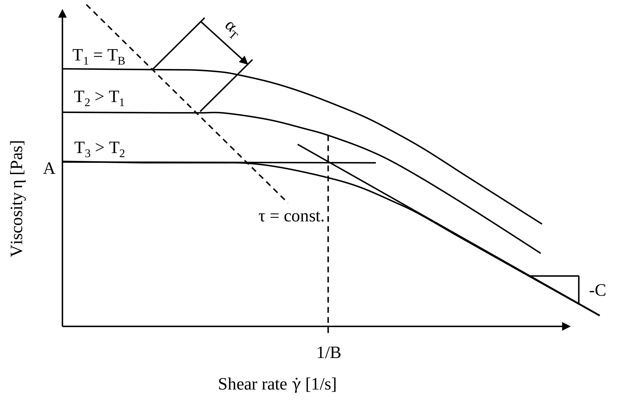
The flow properties of polymers depend on the shear rate and temperature.
Description of shear rate dependence: * Carreau approach
$$η = \frac{A \cdot α_{T}} {(1+B \cdot α_{T} \cdot \dot \gamma)^C}$$
- Yasuda approach
$$η (\dot \gamma, T) = η_∞ \cdot a_T + \frac{A \cdot a_T - η_∞ \cdot a_T} {(1 + (B \cdot a_T \cdot \dot \gamma)^κ)^\frac{1-C}{κ}}$$
- Polynomial approach
$$η = ln (α_0 + α_1 \cdot ln(\dot \gamma) + α_2 \cdot ln(\dot \gamma)^2 + α_2 \cdot T + α_{22} \cdot T^2 + α_{12} \cdot T \cdot ln(\dot \gamma))$$
- Power approach
$$η = K \cdot α_T \cdot \dot \gamma^{n-1}$$
Description of temperature dependence: * WLF (Tb, Ts)
$$log(a_T) = \frac {C_1\cdot(T_B-T_S)} {C_2+(T_B-T_S)} - \frac {C_1\cdot(T-T_S)} {C_2+(T-T_S)}$$
- WLF (C1, C2)
$$ln(a_T) = - \frac {C_1 \cdot (T-T_B)} {C_2+(T-T_B)}$$
- Arrhenius
$$ln(a_T)=\frac{E}{R} (\frac{1}{T+273.15}-\frac{1}{T_B+273.15}) $$
Description of pressure dependence: * Beta
$$β=ln[\frac{η(p2)}{η(p1)}] \cdot \frac{1}{(p2-p1)}$$
In some cases, the regression does not produce a meaningful result. This problem can often be solved by selecting a different reference temperature and/or a different calculation approach. Nevertheless, it should be noted that regression always produces an approximate result, which often cannot provide the desired accuracy for mathematical reasons.
Thermodynamical Data
When evaluating the thermodynamic data and densities, a distinction must be made between whether the molecular structure of the polymer is amorphous or semi-crystalline. Different curves result depending on the molecular structure.
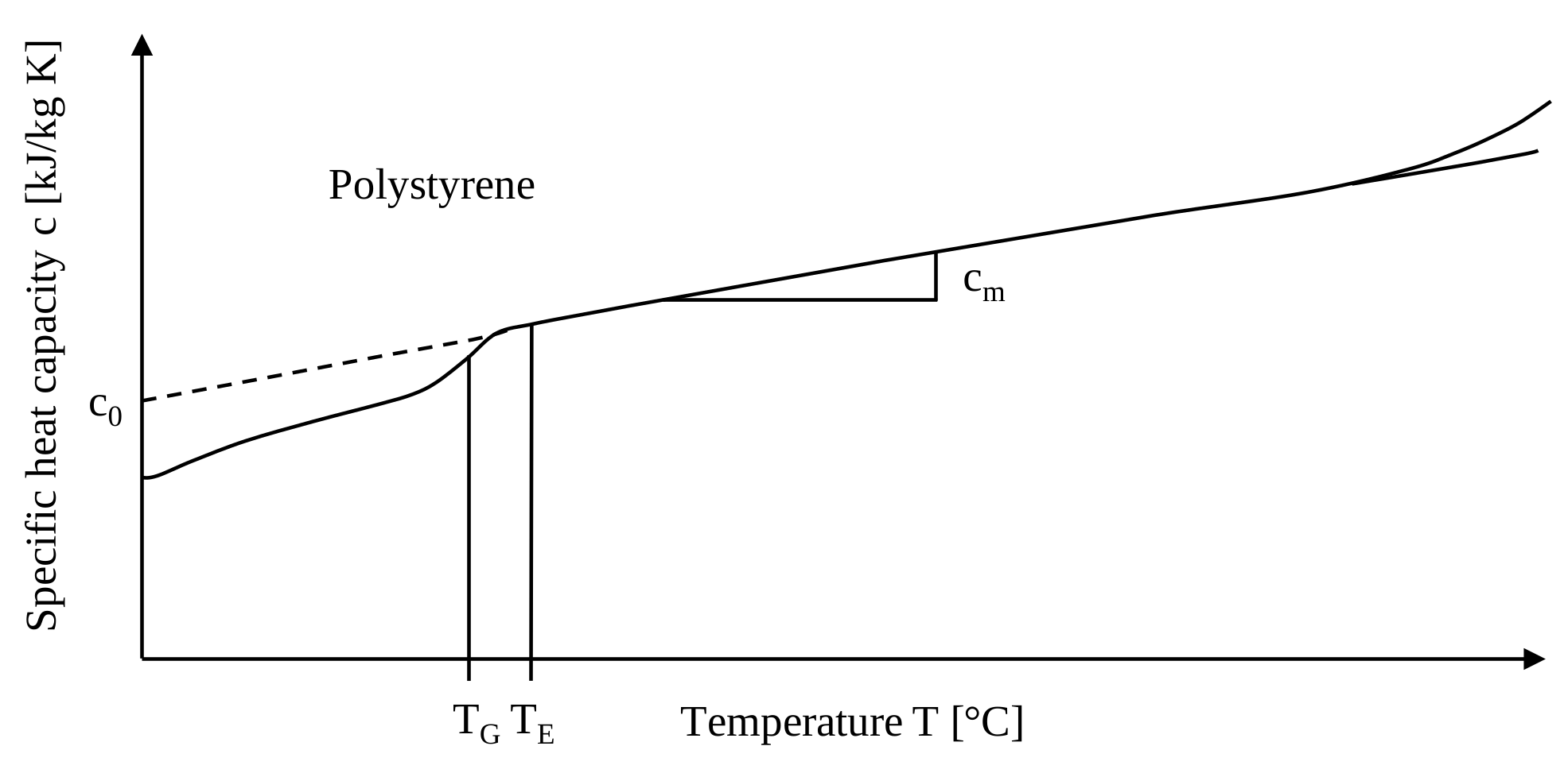
Specific Heat Capacity
- amorphous polymers
- partially crystalline polymers
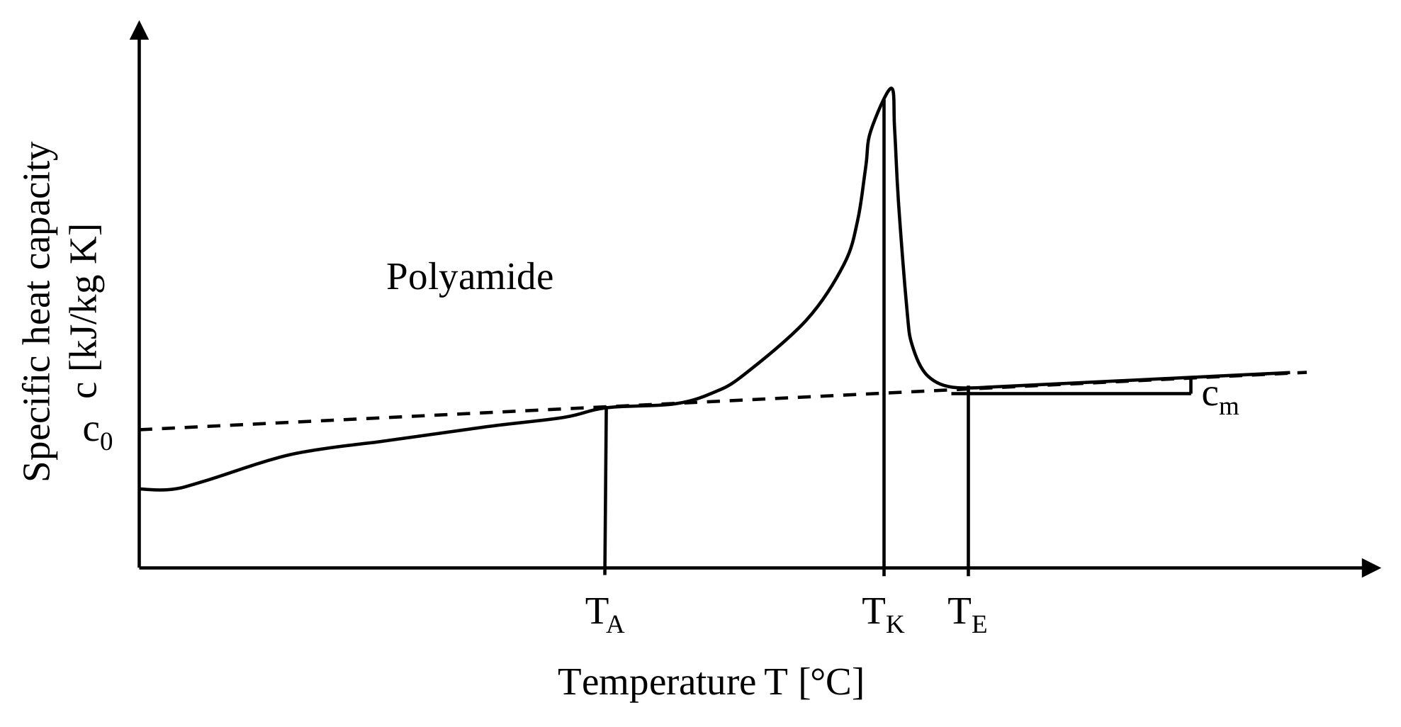
Where there are significant changes in the curve, the characteristic temperature of the material is $Tg$ for amorphous materials and $Tk$ for semi-crystalline materials. To evaluate the material data, first determine the characteristic temperature and then perform a linear regression in the range $T$ »$Tg$ or $Tk$ using the following equation.
$$c_p(T) = c_{p,0} + c_{p,m}\cdot T$$
Enthalpies
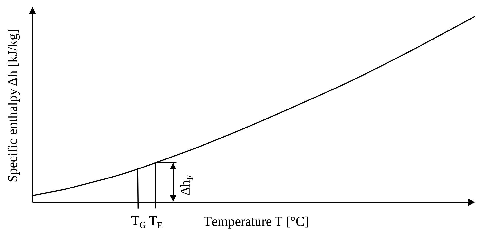
The following enthalpy curves result for amorphous or semi-crystalline materials:
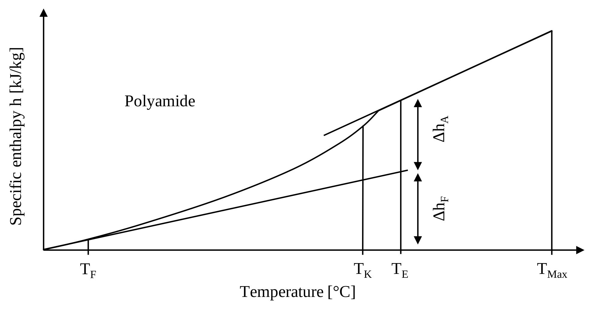
For semi-crystalline materials, a tangent must first be calculated at low temperatures. The enthalpy at this point is then divided into enthalpy components below the tangent, as shown in the following figure, on the one hand into the solid enthalpy $∆h_F$ and on the other hand into the melting enthalpy $∆h_A$.