Dies ist eine alte Version des Dokuments!
Determination of material data
Pure polymers
A thorough knowledge of the material parameters and the behaviour of the material are vitally important to be able to obtain results.
In order to describe the behavior of the polymers, the following properties must be examined:
- Rheological properties (shear viscosity)
- Thermodynamic properties (crystalline melting / glass transition temperature, heat capacity, specific enthalpy, thermal conductivity)
- Density (specific volumes, bulk density, solid material density)
- Size of the pellet granule
Rheological Material Parameters
The behavior of the flow of the fluids is described using the law:
$$τ=η\cdot\dotγ$$
with the shear stress $τ$, viscosity $η$ and shear rate $\dotγ$.
Constant viscosities are usually found only for very small and very high shear rates for polymer melts. More often polymer melts show a pseudo-plastic behavior, which can be described using the power law according to Ostwald and de Waale.
$$τ=K\cdot\dotγ^n$$
Here, $n$ is the exponent of the flow law (n‹1) and $K$ is the consistency factor.
In double logarithmic scale, the viscosity over the shear rate yields a linear pro-file with gradient ($n-1$).The gradient of this straight line is dependent on the shear rate, therefore for the value of $n$ shear rate ranges must always be given. In addition to this the independent shear rate with zero viscosity cannot be described using the power flow law. This difficulty can be solved using the Carreau equation.
The simulation programmes REX / PSI / SIGMA offer two equations to describe the rheological behavior, firstly the Carreau–WLF (Williams, Landel-Ferry) equation and secondly the Carreau-Arrhenius equation. The equations differ in that they offer different descriptions for the dependence of the temperature on the viscosity. This difference was introduced so that data from different origins (CAMPUS; BAYMAT; VISCOSITY) are able to be entered without conversions. The evaluation of the viscosity function with the Carreau-estimation program offers not only the zero viscosity $a$, but the reciprocal transitional shear rate $b$, the gradient $c$, the reference temperature $T_b$ and the standard temperature $T_s$ which are necessary for the following equation:
WLF approach:
$$log(a_T) = \frac {C_1\cdot(T_B-T_S)} {C_2+(T_B-T_S)} - \frac {C_1\cdot(T-T_S)} {C_2+(T-T_S)}$$
with: $C_1$ = 8.86, $C_2$ = 101.6, $T_B$ = reference temperature, $T_S$ = standard temperature ($T_S ≈ T_G + 50°C$), $T$ = current temperature
The WLF equation provides a better description than the Arrhenius approach, especially for amorphous polymers whose molten state begins at a temperature slightly above the glass transition temperature. This assumes that the segment mobility of polymers near the glass transition temperature is primarily determined by the free volume, which increases approximately linearly with the distance from the glass transition temperature TG. It is assumed that the segment mobility of polymers near the glass transition temperature is predominantly determined by the free volume, which increases approximately linearly with the distance from the glass transition temperature TG [Fer80]. If a temperature approximately 50°C above the glass transition temperature $T_G$ is selected as the standard temperature $T_S$, the parameters $C_1$ and $C_2$ in the equation can be regarded as material-independent [Mel95].
Alternatively, the following approach can also be used:
$$ln(a_T) = - \frac {C_1 \cdot (T-T_B)} {C_2+(T-T_B)}$$
with: $T_B$ = reference temperature, $T$ = current temperature, $C_1$ = adjustment constant, $C_2$ = adjustment constant
can also be used.
The Arrhenius approach, which is also available, is:
$$ln(a_T)=\frac{E}{R} (\frac{1}{T+273.15}-\frac{1}{T_B+273.15}) $$
where: $T_B$ = reference temperature, $T$ = current temperature, $E$ = activation energy, $R$ = universal gas constant
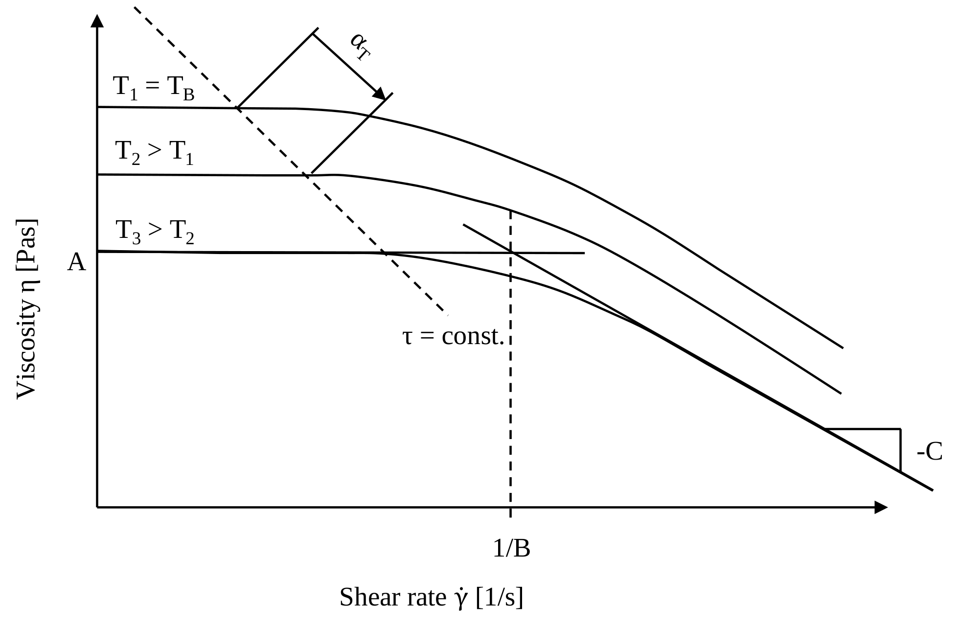
Measuring Series with the High Pressure Capillary Rheometer
In order to be able to define the necessary Carreau parameters, measurements have to be taken, for instance, with the high-pressure capillary rheometer. Usually the experimental series are performed at 3 different temperatures.
In a high-pressure capillary rheometer, pre-heated material flows through a capillary with a circular cross-section. During this process, the total area of the important viscosities is measured. For low viscosity fluids, long thin capillaries are used and for high viscosity fluids appropriately high pressures are used. By using this discontinuous method, the necessary pressure is made available through carrier gas, gravity or by means of pistons. The volume flow rate is constant at a constant piston speed. The pressure gradient at the inlet and at the outlet is not constant due to vortex formation as a result of viscoelastic effects (Bagley-Correction), due to the change of the flow speed (Hagenbach-Correction) and due to the variation of the friction at the wall (Couette-Correction). To calculate the exact viscosity of the polymer melt, the pressure gradient is measured using two pressure sensors on a designated length in the capillary, because here are simple rheological flow relationships.
Thermodynamic Material Parameters
The calculation of both the melting behavior and the temperature development in power melts requires a comprehensive knowledge of the thermodynamic material behavior [Hen89]. The thermodynamic properties are dependent on both pressure and temperature and show a different material property in the solid state and in the melt state.
The following data is required for REX / PSI / SIGMA: the crystalline melting temperature, glass transition temperature, specific heat capacity and specific enthalpy. These can be detected using the DSC (Difference Scanning Calorimetric)- analysis.
General Principle of the DSC-Analysis
The principle is based on the measurement of the heat flow between one specimen and a comparable substance in a twin calorimeter. The sample and the reference substances are arranged symmetrically to each other so that the temperature difference is zero. Many chemical and physical transitions like melting, crystallisation, oxidation or decomposition of a substance are related to a heat flow i.e. changes in enthalpy appear. These enthalpy changes are detected by the DSC-analysis with regard to their position in the temperature range and their calorimetric magnitude. The specific heat and the enthalpy as a function of temperature can be quantified very quickly and very easily. The measurement principle is shown in the following figure.
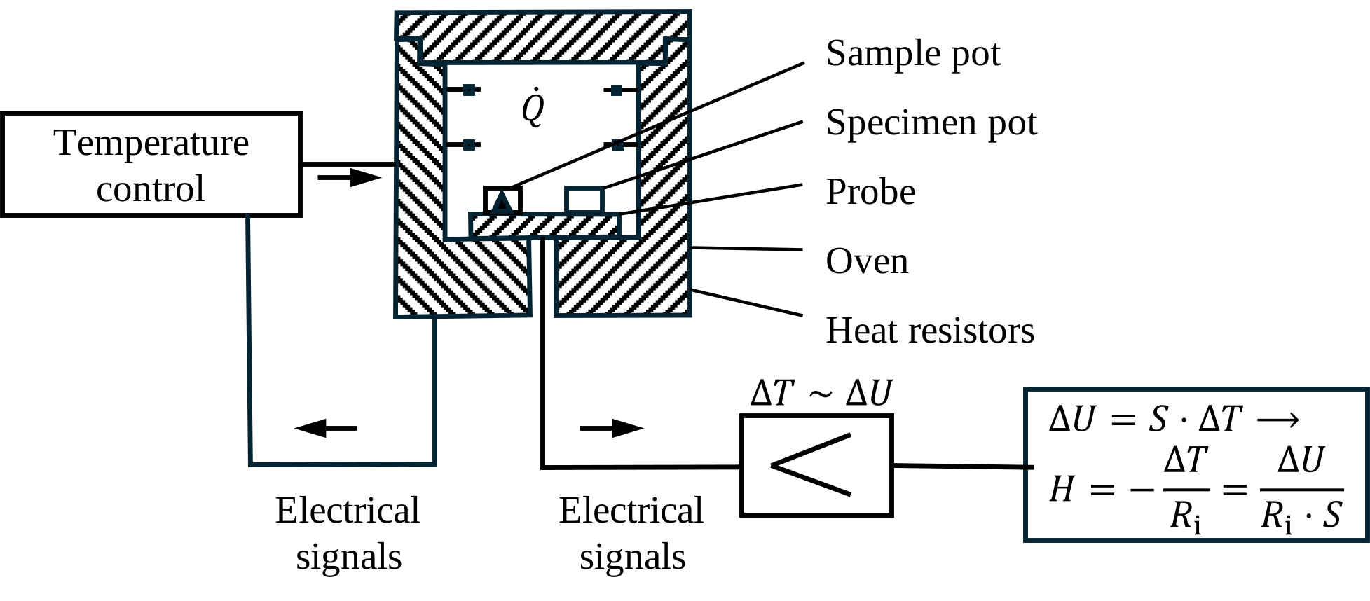
Through a temperature sensor designed as a thermal resistor, a heat flow $\dot Q$ is conducted from the electrically heated furnace body to both the sample crucible and the reference crucible, which are usually identical (same dimensions, same material). The heat flow to the reference crucible $\dot Q_R$ is determined by the heat capacity of the crucible material and the inherent thermal losses.
This also applies to the sample crucible in the case of identical crucible materials and a symmetrical measuring cell. However, the specimen enclosed in the sample crucible ($\dot Q_S = \dot Q_R$) generates an additional heat flow $\dot H$ ($dH/dt$), which can now be determined by difference calculation:
$$\dot H = \dot Q_S - \dot Q_R = \frac{T_P-T_S}{R_t} - \frac{T_P-T_R}{R_t} = \frac{T_S-T_R}{R_t} = - \frac{ΔT}{R_t}$$
Here, $\dot H$ = heat flow of the specimen, $\dot Q_S$ and $\dot Q_R$ = heat flow to the sample and reference crucible, $R_T$ = thermal resistance of the sensor, $T_P$ = furnace temperature (temperature program), and $T_S$ and $T_R$ = sample and reference temperature.
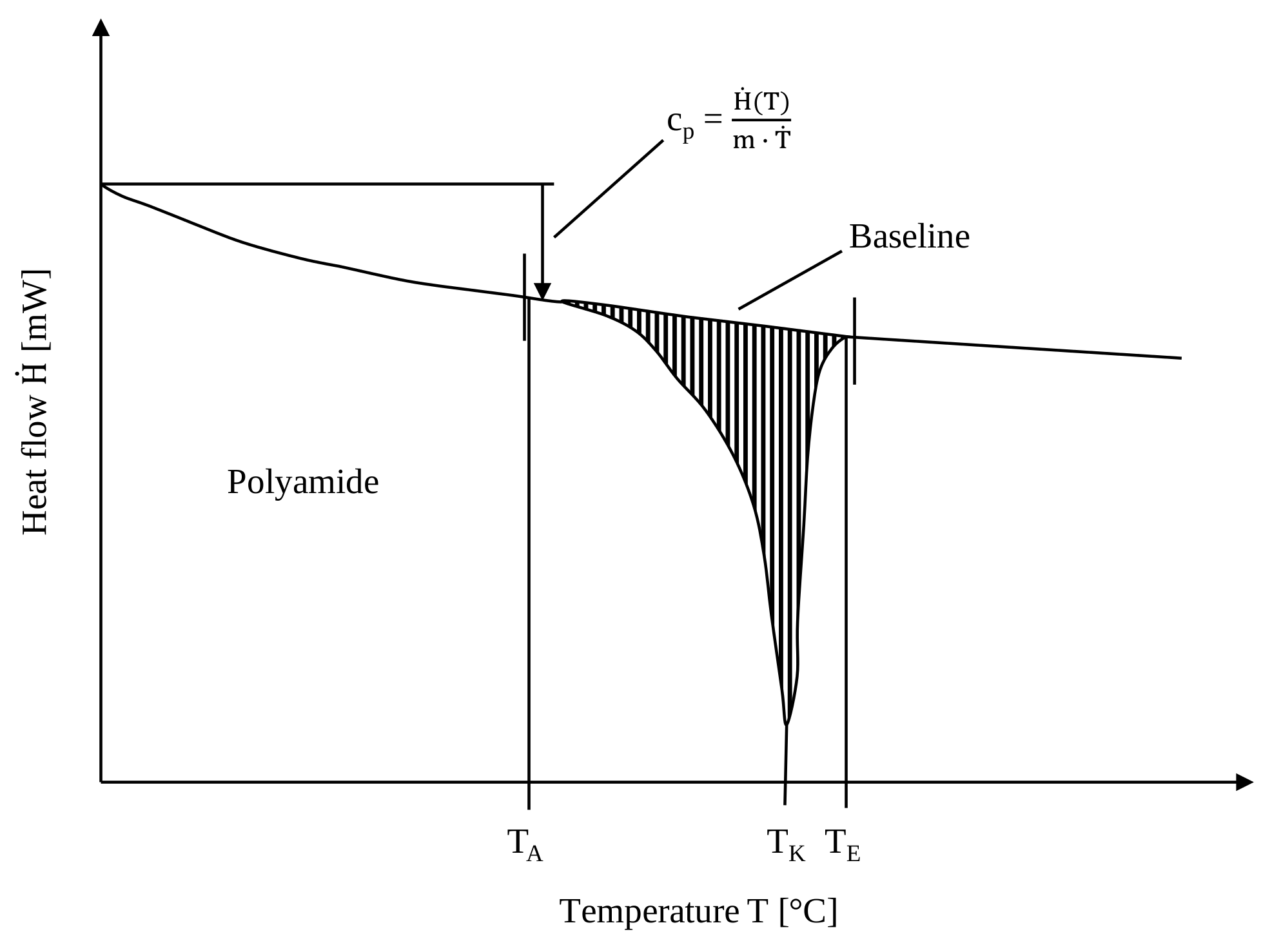
Semi-crystalline thermoplastics do not exhibit a sharp melting point like metals but rather a melting range, due to the presence of crystallites of different lamellar thicknesses. Smaller, less perfectly ordered crystallites melt at lower temperatures than larger crystallites. A characteristic feature of every semi-crystalline polymer material is the melting or crystallite peak temperature $T_K$. The position of this peak on the temperature axis is defined by the onset temperature ($T_A$), the peak temperature ($T_K$), and the end temperature ($T_E$), which are also of importance when determining other thermodynamic properties, such as the specific enthalpy.
When plotting the heat flow $\dot H (T)$ as a function of temperature $T$, semi-crystalline thermoplastics exhibit the following characteristic profile.
Description of Thermodynamic Material Properties
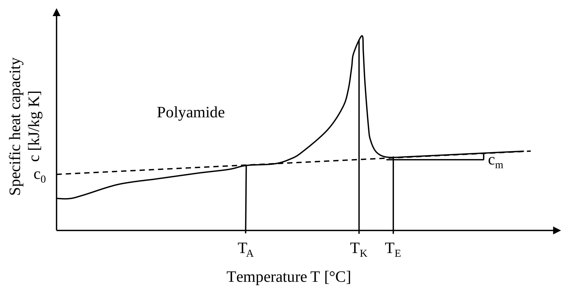
The specific heat capacity $c$ of polymers typically lies in the range of 0.1 to 5 kJ/kg K. The following figure illustrates, as an example, the temperature dependence of the specific heat capacity $c$ for a semi-crystalline polyamide.
Amorphous polymers exhibit a different heat capacity profile $c(T)$ compared to semi-crystalline polymers. At the glass transition temperature $T_G$, a distinct change in the level of the specific heat capacity $c$ can be observed.
The next figure shows the specific heat capacity $c$ as a function of temperature for an amorphous polystyrene.
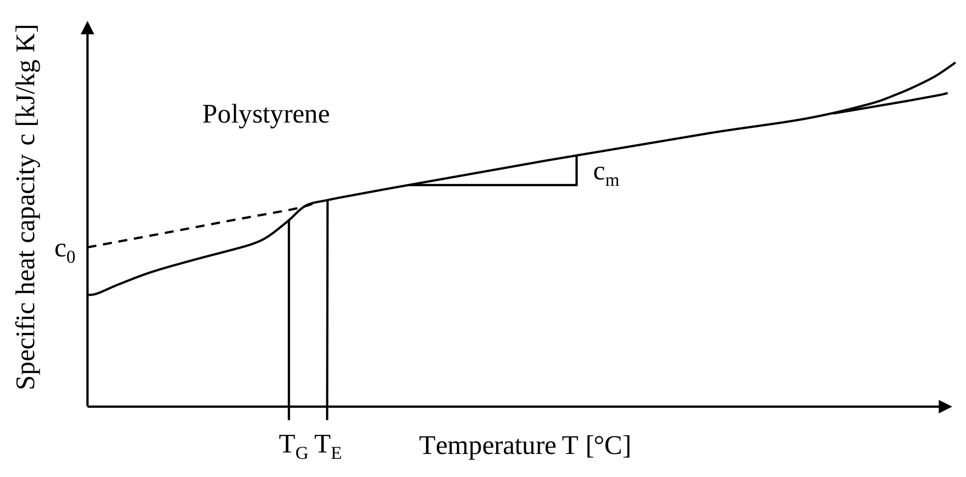
For simulation purposes with REX / PSI / SIGMA, the material data obtained from DSC analysis are approximated above the melting end temperature or the end temperature of the softening range $T_E$ by a linear function, as indicated by the dashed lines in the thermograms above:
$$c_p(T) = c_{p,0} + c_{p,m}\cdot T$$
In this function, the index $0$ denotes the material property at $0 °C$, while the index $m$ represents the slope of the property function.
Since REX / PSI / SIGMA does not account for pressure effects, the determination of the thermodynamic material properties should always be performed at a mean pressure [Mel95].
The specific enthalpy $∆h$ results from the integration of the specific heat capacity $c$ over the temperature range between $T_1$ and $T_2$, which can be derived from DSC analysis. In this way, the amount of heat per unit mass of the polymer that must be supplied is obtained. The following relation applies:
$$Δh = \int \limits_ {T_1}^{T_2} c_p(T)dT$$
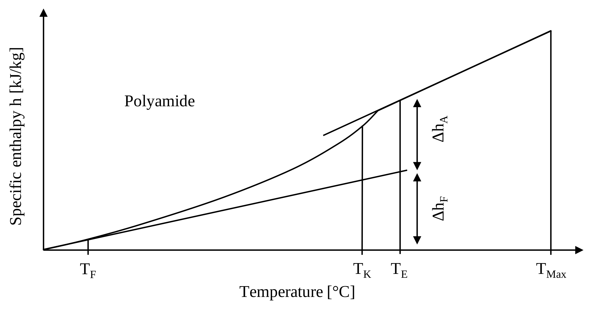
For simulations with REX / PSI / SIGMA, the functional relationship of specific enthalpy $∆h$ over temperature $T$ is not of primary interest. Instead, the characteristic values for semi-crystalline polymers or blends, such as the solid enthalpy $∆h_F$ and the melting enthalpy $∆h_A$, are required.
The determination of these parameters is exemplified below using a semi-crystalline polyamide. The melting process is initiated by the supply of heat (latent heat of fusion) into the system and is completed upon reaching the end temperature $T_E$. The total enthalpy difference observed at this temperature corresponds to the energy required to completely melt the polymer.
By constructing tangents in the lower and upper temperature ranges, this total enthalpy $∆h$ can be separated into the partial enthalpies $∆h_F$ and $∆h_A$. In the lower temperature range, a suitable approximation can be achieved with statistical software by comparing the coefficients of determination for different interval widths [$T_F$ ; $T$]. In the upper temperature range, the interval [$T_E$ ; $T_{MAX}$] serves as the basis for tangent determination.
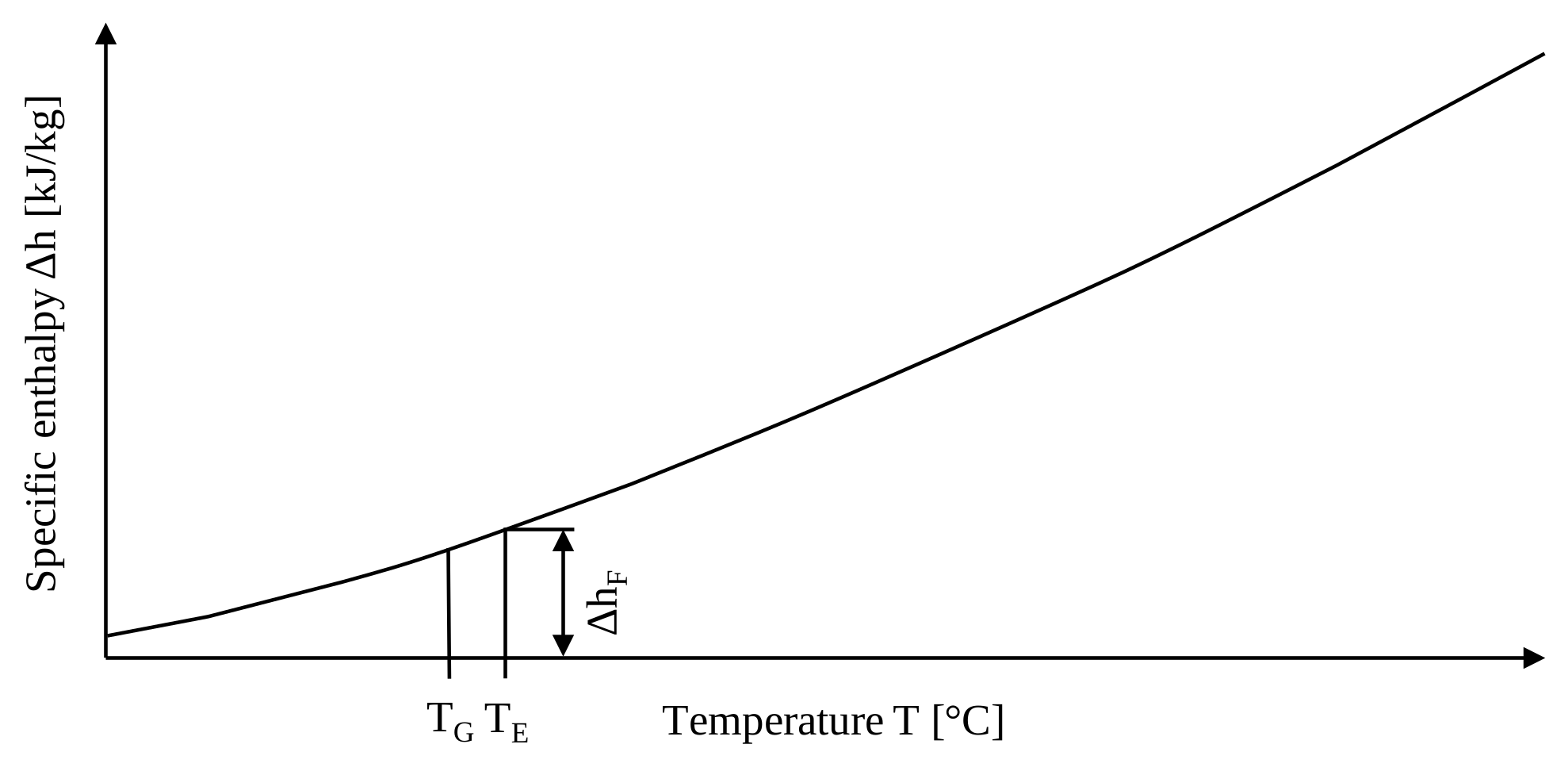
Amorphous systems, by contrast, show a fundamentally different enthalpy behavior due to the absence of a melting transition. For each amorphous polymer, only the solid enthalpy $∆h_F$ is used as a characteristic value. This corresponds to the enthalpy level at the end of the softening range, at the end temperature $T_E$.
The following figure illustrates, as an example, the determination of the solid enthalpy $∆h_F$ for an amorphous polystyrene.
Thermal Conductivity
In heat conduction processes, a distinction is made between steady-state and non-steady-state temperature fields. In steady-state temperature fields, the thermal conductivity $λ$ appears as a material property. It is temperature dependent and lower for amorphous materials than for semi-crystalline ones [Mel95].
The determination of the thermal conductivity $λ$ can, for example, be carried out using a Thermoflixer device manufactured by SWO Polymertechnik. The measuring principle is illustrated in the following figure.
The measurement is performed in a heated test chamber containing a defined specimen mass $m$ and a sensor in direct contact with the sample. Over a defined measuring period $t$, an energy amount $\dot Q$ is supplied to the specimen.
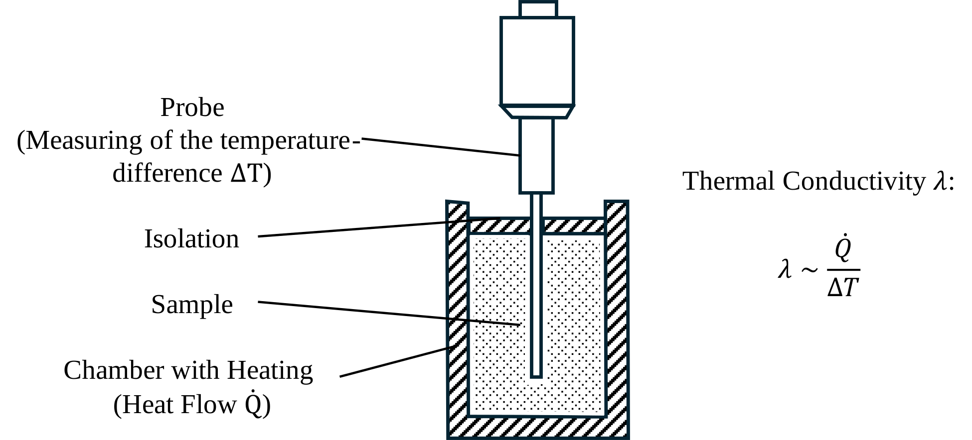
The temperature change $∆T$ experienced by the specimen during this measuring period is detected by the sensor. From the supplied heat $Q$ and the measured temperature change $∆T$, the thermal conductivity $λ = f(\dot Q , ∆T)$ can be determined. The advantage of this measuring principle compared to the plate method according to DIN 52 612 lies in its ability to measure thermal conductivities $λ$ even at very high temperatures, which are of particular importance for polymeric materials.
The next figure shows a typical course of thermal conductivity $λ$ as a function of temperature $T$ for semi-crystalline polymers, using polypropylene as an example.
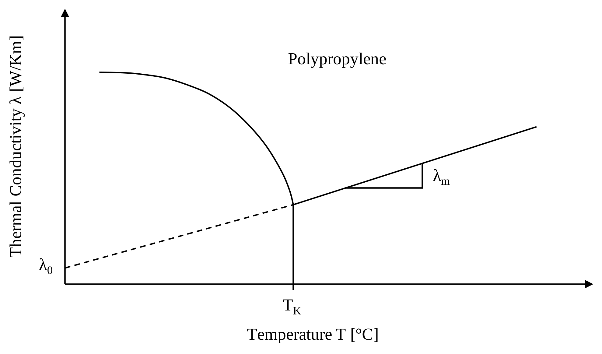
For simulation purposes, a linear equation of the form
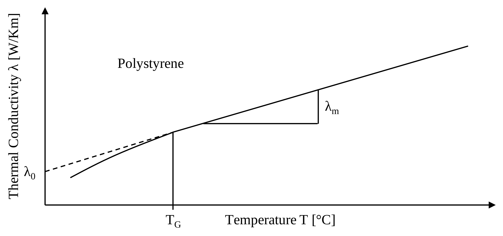
$$λ(T) = λ_0 + λ_m \cdot T$$
is required, according to the dashed line shown in the figure. The parameters to be determined are the specific thermal conductivity at $0 °C$ ($λ_0$) and the slope of the thermal conductivity function ($λ_m$).
The temperature dependence of the thermal conductivity $λ$ for an amorphous polystyrene is also shown for comparison.
Melting Temperature
In the evaluation of DSC analyses, the supplied energy is plotted as a function of temperature. For semi-crystalline thermoplastics, the crystallization temperature $T_K$ can be determined from the peak maximum of the curve. In the case of amorphous thermoplastics, the glass transition temperature $T_G$ can be obtained from the inflection point of the curve.
Densities
When plotting the specific volume $v$ as a function of temperature $T$ for a semi-crystalline polymer, it becomes evident that the behavior over the entire temperature range can only be described mathematically with difficulty, if at all.
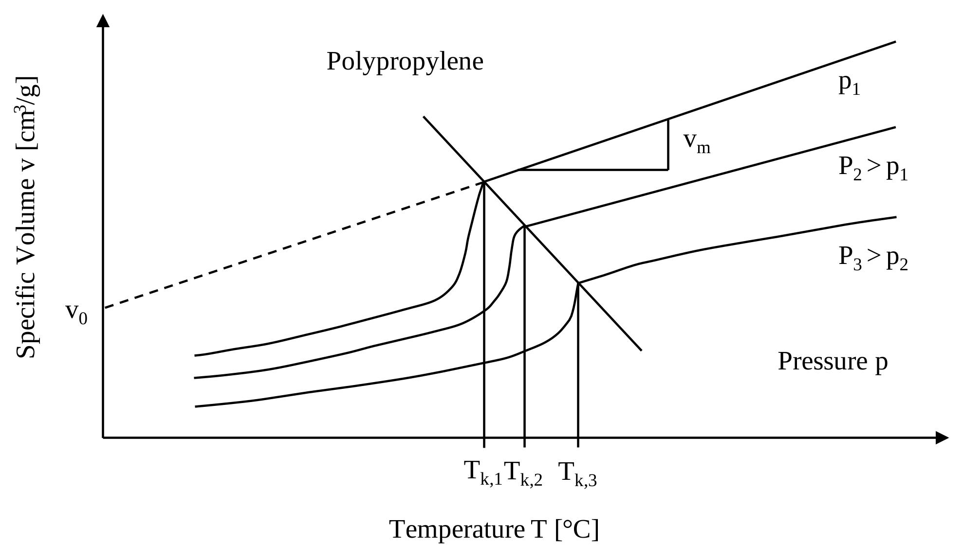
The following figure additionally shows the specific volume $v$ as a function of temperature $T$ for an amorphous polystyrene.
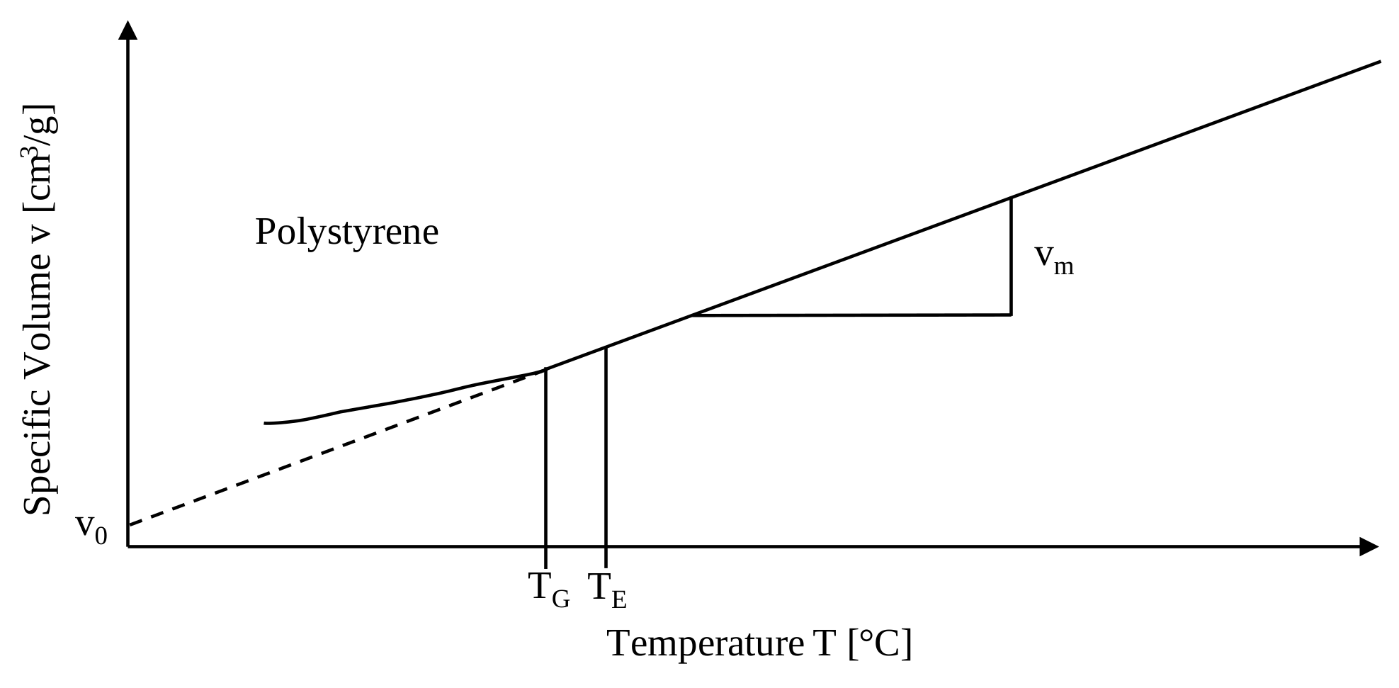
For the simulation of melt-dominated extruders, however, the primary interest lies in the temperature range above the melting temperature $T_K$ or the glass transition temperature $T_G$. REX / PSI / SIGMA requires a description of the volume or density function in the following form:
$$v(T) = v_0 + v_m \cdot T$$ $$ρ(T) = ρ_0 - ρ_m \cdot T$$
where: $v_0$ = specific volume $v_m$ = slope of the volume function $ρ_0$ = specific density $ρ_m$ = slope of the density function
The procedure for determining the bulk density $ρ_s$ is defined in DIN 53 466.
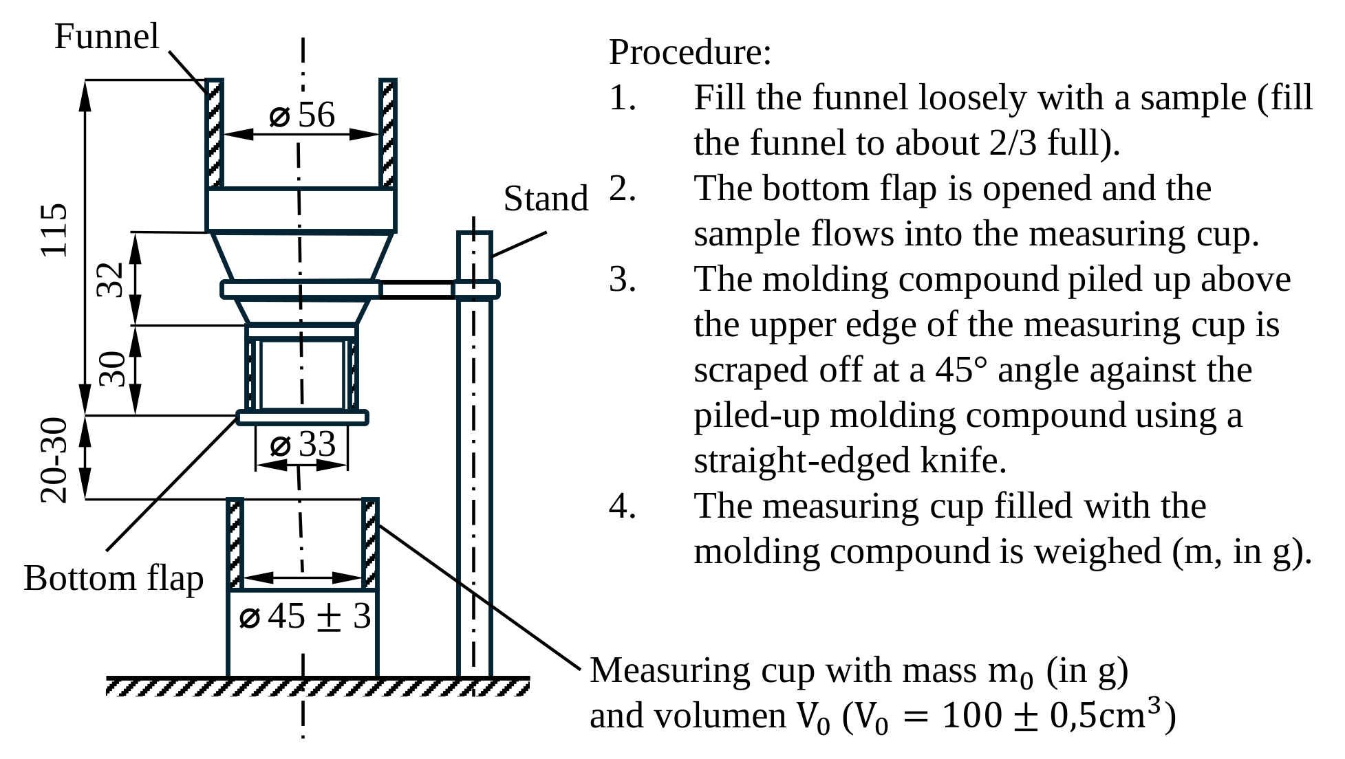
The bulk density $ρ_s$ is mainly used to determine the maximum mass throughput $\dot m$ of the system and the filling degree $f$ in the solids conveying section. For example, the required screw speed range for a given throughput can be calculated, or conversely, the maximum possible throughput can be determined at a specified screw speed. The evaluation is carried out according to the following equation:
$$ρ_s = \frac{m_1 - m_0}{V_0}$$
with $m_1$ = mass of the container filled with the specimen, $m_0$ = mass of the empty container, and $V_0$ = volume of the container
The solid densities can be determined according to DIN 53 479. This method (buoyancy method) compares the weight of a defined sample mass in air with its apparent weight in a liquid medium (here: distilled water, $ρ_{H_2O}$ = 1.000 g/cm³).
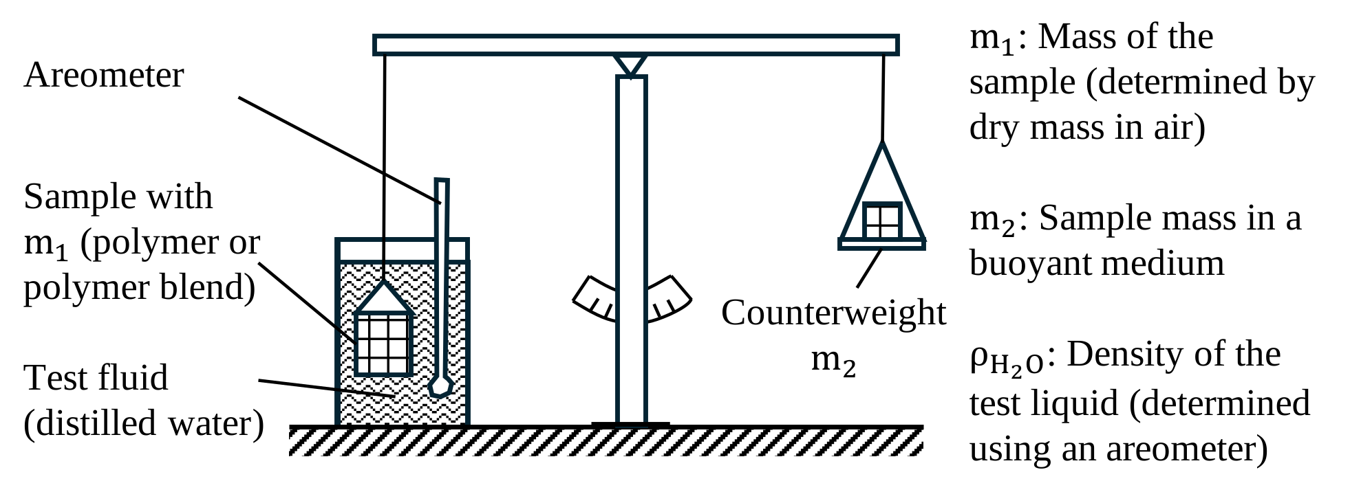
For the solid density of the specimen, the following relation applies:
$$ρ = \frac{m_1 \cdot ρ_{H_2O}}{m_1 - m_2}$$
where $m_1$ = dry mass in air and $m_2$ = specimen mass in the buoyant medium.
Pellet Size
For the determination of pellet size, the specimens are first averaged volumetrically from a total of $n$ pellets and subsequently converted into spherical form. The determination of the pellet size is illustrated schematically in the following figure and can be derived from the relation:
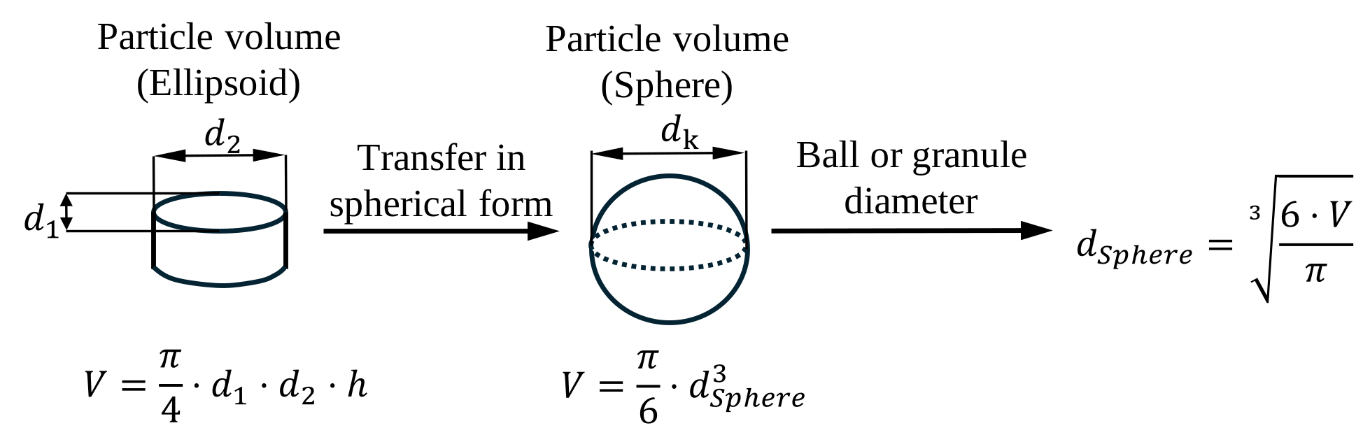
An alternative approach is to calculate the pellet diameter $d$ from a total of $n$ specimens using the solid density $ρ$ and the total mass of the specimens $m_{ges}$. For the total of $n$ specimens, the following holds:
$$V_{ges} = \frac{m_{ges}}{ρ}$$
For a single averaged pellet, this results in:
$$V = \frac{V_{ges}}{n}$$
The pellet diameter $d_{sphere}$ can then be determined using the following equation.
References
[Fer80]
[Hen89]
[Mel95]
Mixture rules for polymer blends
The rheological as well as the thermodynamic parameters of two-component systems (e.g., solidification and melting enthalpies of polymer blends) generally cannot be determined with sufficient accuracy by a simple linear averaging of the data of the base components. For simulations with REX / PSI / SIGMA, this means that, prior to the actual simulation runs, complete material data for the polymer blends should ideally be determined experimentally. However, this requires a considerable amount of measurements even before the simulation process itself can be carried out. If, on the other hand, only the material data of the individual components are available, the material data of the blends are calculated within REX / PSI / SIGMA from the component data as follows.
Rheological Parameters of Multicomponent Systems
For calculating the viscosity of two-phase polymer blends, the literature provides a range of mixing rules that vary in complexity depending on the required level of accuracy—from simpler approaches to more mathematically elaborate ones. In the simulation software packages REX / PSI / SIGMA, the following general mixing rules are applied:
first, the simplest and most widely used logarithmic mixing rule according to Arrhenius:
$$log η_{MIX} = w_1 \cdot log η_1 + w_2 \cdot log η_2$$
and second, the mixing rule proposed by Mantford:
$$(η_{MIX})^{1/3,4} = w_1 \cdot η_1^{1/3,4} + w_2 \cdot η_2^{1/3,4}$$
The determination of the blend viscosity from the viscosities of the individual components $η_i$ and their weight fractions $W_i$ using REX / PSI / SIGMA is illustrated in the following figure.
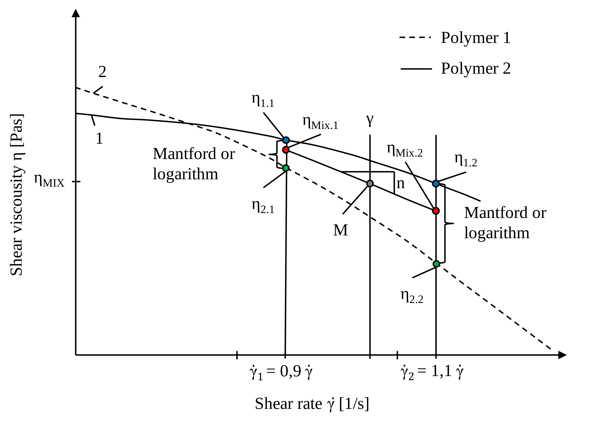
To calculate the viscosity $η_{MIX}$ at a given shear rate $\dot γ$ for a polymer blend, the blend viscosities $η_{MIX1}$ and $η_{MIX2}$ are first determined for the defined shear rates $\dot γ_1 = 0.9 \cdot \dot γ$ and $\dot γ_2 = 1.1 \cdot \dot γ$. For the Mantford approach, the following applies:
$$(η_{MIX1})^{1/3,4} = w_1 \cdot η_1.1^{1/3,4} + w_2 \cdot η_2.1^{1/3,4}$$ $$(η_{MIX2})^{1/3,4} = w_1 \cdot η_1.2^{1/3,4} + w_2 \cdot η_2.2^{1/3,4}$$
Analogously, the logarithmic mixing rule (Arrhenius) is given by:
$$log η_{MIX1} = w_1 \cdot log η_1.1 + w_2 \cdot log η_2.1$$ $$log η_{MIX2} = w_1 \cdot log η_1.2 + w_2 \cdot log η_2.2$$
If these quantities are known, the flow behavior index $n$ and the consistency $K$ of the approximated blend segment between $\dot γ_1 = \dot γ_{MIX1}$ and $\dot γ_2 = \dot γ_{MIX2}$ can be determined as follows:
$$n = 1 + \frac{log(\frac{η_{MIX1}}{η_{MIX2}})}{log(\frac{\dotγ_{MIX1}}{\dotγ_{MIX2}})}$$
$$K = \frac{η_{MIX1}}{\dotγ_{MIX1}^{n-1}}$$
The desired viscosity $η_{MIX}$ is finally obtained by:
$$η_{MIX} = K \cdot \dotγ_{MIX}^{n-1}$$
If the dispersed phase is present in solid or highly viscous form, the system can be regarded as a filled polymer. For simulation purposes, in the case of a filled polymer the base polymer and its particle diameter must first be defined. The filler is then specified. This requires a range of material data: the particle diameter $d$, the mass fraction $w$, the solid density $ρ$, the bulk density $ρ_s$, the thermal conductivity of the solid $λ_0$, and the specific heat capacity $c_0$. Similar to polymer blends, two mixing equations are also available for filled polymers. The first is the simple approach according to Einstein:
$$η_{MIX} = η_1 \cdot (1 + 2,5 \cdot Φ_2)$$
and finally, the approach according to Hashin:
$$η_{MIX} = η_1 \cdot [1+2 \cdot \frac{Φ_2}{1-Φ_2}]$$
In these equations, $η_1$ denotes the viscosity of the base polymer, and $Φ_2$ the volume fraction of the added component.
Thermodynamic Parameters of Multicomponent Systems
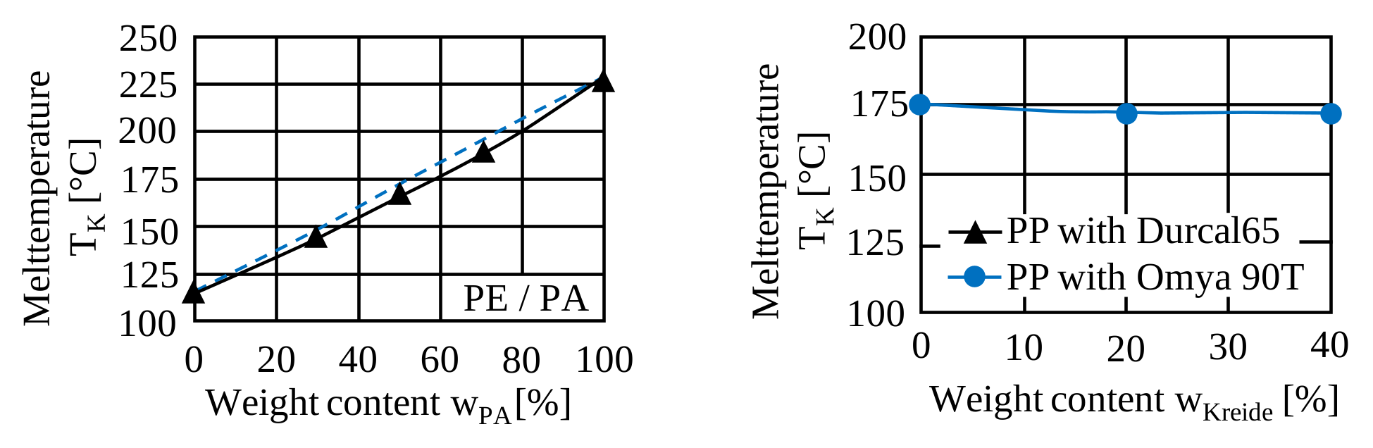
Experimentally determined crystalline melting temperatures, both for polymer blends and for filled systems (compounds), are shown in the following figure. For polymer blends, the crystalline melting temperature $T_{K.MIX}$ is calculated in REX / PSI / SIGMA from the weight fractions $w_i$ and the crystalline melting temperatures $T_{Ki}$ as follows:
$$T_{K.MIX} = w_1 \cdot T_{K.1} + w_2 \cdot T_{K.2}$$
whereas for compounds, the following applies:
$$T_{K.MIX} = T_{K.1}$$
The crystalline melting temperature $T_{K.MIX}$ of a filled polymer (compound) is therefore assumed to be equal to the crystalline melting temperature $T_{K1}$ of the base polymer.
To describe the specific heat capacity $c$ of multicomponent systems, a uniform mixing rule is applied for both polymer blends and filled systems. For the specific heat capacity of the mixture $c_{MIX}$, the following applies:
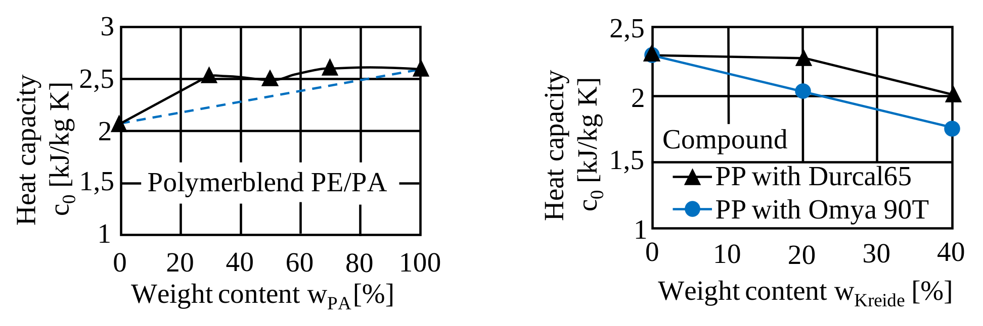
$$c_{MIX} = w_1 \cdot c_1 + w_2 \cdot c_2$$
where $w_i$ are the weight fractions and $c_i$ the specific heat capacities of the individual or added components.
The specific heat capacity $c_{0.MIX}$ of the mixture is therefore given by:
$$c_{0.MIX} = w_1 \cdot c_{0.1} + w_2 \cdot c_{0.2}$$
The following figure shows the course of the specific heat capacity $c_0$ for polymer blends and filled systems. The slope of the heat capacity curve, $c_{m.MIX}$, for the mixture is determined for both systems analogously according to the following equation:
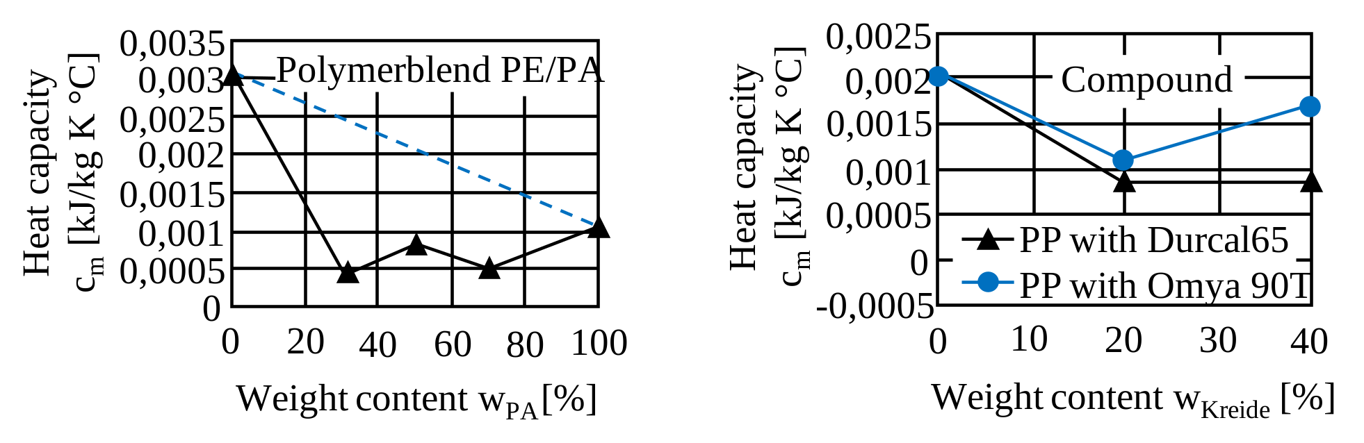
$$c_{m.MIX} = w_1 \cdot c_{m.1} + w_2 \cdot c_{m.2}$$
The relationship between the specific heat capacity $c_m$ and the weight fractions for polymer blends and filled systems is illustrated as an example:
The specific enthalpy is given by:
$$Δh = w_1 \cdot Δh_1 + w_2 \cdot Δh_2 = w_1 \cdot {(Δh_F + Δh_A)}_1 + w_2 \cdot {(Δh_F + Δh_A)}_2$$
Index 1 refers to polymer 1 and index 2 to polymer 2.
For describing the specific enthalpy $Δh$ of filled systems (compounds), the following approach is used:
$$Δh = w_1 \cdot {(Δh_F + Δh_A)}_1 + w_2 \cdot c_2 \cdot ΔT$$
Here, index 1 refers to the polymer, while index 2 denotes the filler.
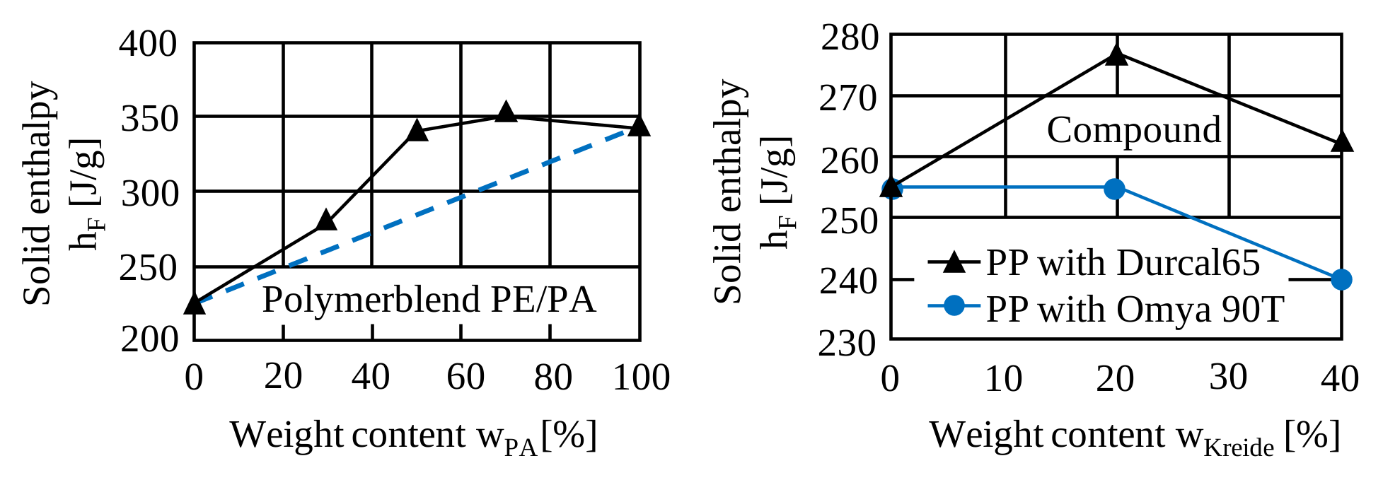
The solid enthalpy $Δh_F$ and melting enthalpy $Δh_A$ for polymer blends can be determined from the enthalpy values of the individual components as follows. For the solid enthalpy $Δh_{F.MIX}$ and melting enthalpy of the mixture $Δh_{A.MIX}$:
$$Δh_{F.MIX} = w_1 \cdot Δh_{F.1} + w_2 \cdot Δh_{F.2}$$
$$Δh_{A.MIX} = w_1 \cdot Δh_{A.1} + w_2 \cdot Δh_{A.2}$$
Analogously, for compounds (filled systems), the solid enthalpy $Δh_{F.MIX}$ and melting enthalpy $Δh_{A.MIX}$ of the mixture are calculated as follows:
$$Δh_{F.MIX} = w_1 \cdot Δh_{F.1}$$
$$Δh_{A.MIX} = w_1 \cdot Δh_{A.1} + w_2 \cdot c_2 \cdot ΔT$$
The following figures show, as examples, results from experimental investigations of the specific solid enthalpy $Δh_F$ and specific melting enthalpy $Δh_A$ of multicomponent systems.
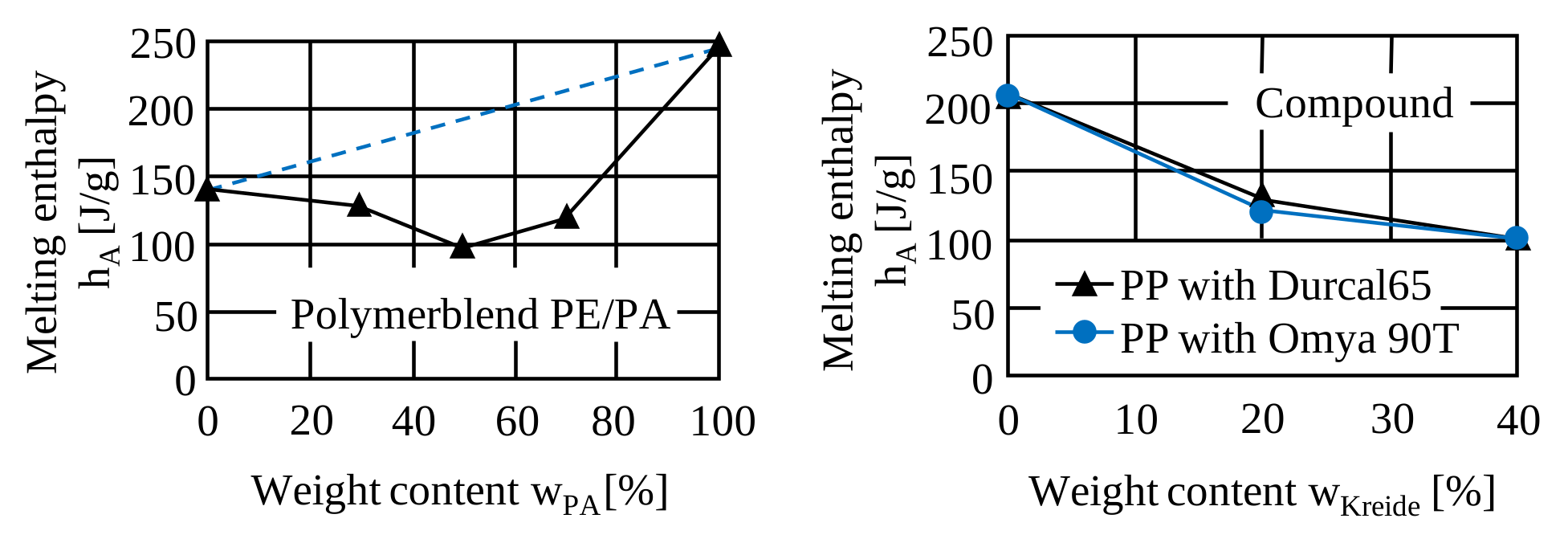
In the simulation programs REX / PSI / SIGMA, the following equations are used to determine the thermal conductivity $λ_{MIX}$ of multicomponent systems from the values of the individual polymers ($w_i$, $λ_i$). For polymer blends:
$$λ_{MIX} = w_1 \cdot λ_1 + w_2 \cdot λ_2$$
For filled polymers (compounds), the following relationship is assumed for calculating the thermal conductivity:
$$λ_{MIX} = λ_2 \cdot \frac{λ_1 + 2 \cdot λ_2 - 2 \cdot Φ_1 \cdot (λ_2 - λ_1)}{λ_1 + 2 \cdot λ_2 + Φ_1 \cdot (λ_2-λ_1)}$$
While indices 1 and 2 correspond to the individual polymers 1 and 2 in polymer blends, for filled systems index 1 refers to the base polymer and index 2 to the added filler. For each component, the linear approximation is applied:
$$λ_i = λ_{0.i} + λ_{m.i} \cdot T$$
Here, $λ_{0.i}$ is the value of the linear approximation for the thermal conductivity of a component at $T = 0°C$, while $λ_{m.i}$ is the slope of the approximated thermal conductivity curve of the component above the melting temperature. For polymer blends, the thermal conductivity of the mixture $λ_{0.MIX}$ is:
$$λ_{0.MIX} = w_1 \cdot λ_{0.1} + w_2 \cdot λ_{0.2}$$
The slope of the mixture’s thermal conductivity function $λ_{m.MIX}$ is calculated as:
$$λ_{m.MIX} = w_1 \cdot λ_{m.1} + w_2 \cdot λ_{m.2}$$
For filled polymers (compounds), the following mixing equations are used to determine $λ_{0.MIX}$ and $λ_{m.MIX}$:
$$λ_{0.MIX} = λ_{0.2} \cdot \frac{λ_{0.1} + 2 \cdot λ_{0.2} -2 \cdot Φ_1 \cdot (λ_{0.2} - λ_{0.1})}{λ_{0.1} + 2 \cdot λ_{0.2} + Φ_1 \cdot (λ_{0.2} - λ_{0.1})}$$
and
$$λ_{m.MIX} = λ_{m.2} \cdot \frac{λ_{m.1} + 2 \cdot λ_{m.2} -2 \cdot Φ_1 \cdot (λ_{m.2} - λ_{m.1})}{λ_{m.1} + 2 \cdot λ_{m.2} + Φ_1 \cdot (λ_{m.2} - λ_{m.1})}$$
Densities of Multicomponent Systems
The calculation of the solid and melt density $ρ_{MIX}$ of polymer blends and compounds from the densities $ρ_i$ and weight fractions $w_i$ of the individual polymers or of the base polymer and filler follows the same equation:
$$\frac {1}{ρ_{MIX}} = \frac{w_1}{ρ_1} + \frac{w_2}{ρ_2}$$
The specific volume $v$ of polymer blends and compounds from the specific volumes $v_i$ and weight fractions $w_i$ of the individual polymers or of the base polymer and filler is calculated using:
$$v_{MIX} = w_1 \cdot v_1 + w_2 \cdot v_2$$
For polymer blends and filled polymers (compounds), the mixture values $v_{0.MIX}$ and $v_{m.MIX}$ are determined using:
$$v_{0.MIX} = w_1 \cdot v_{0.1} + w_2 \cdot v_{0.2}$$
and
$$v_{m.MIX} = w_1 \cdot v_{m.1} + w_2 \cdot v_{m.2}$$
To determine the bulk density $ρ_{S.MIX}$ of multicomponent systems such as polymer blends and compounds with granule diameters $d_1$ and $d_2$ (where $d_1 < d_2$) of the individual components or of the base polymer and filler, some considerations must first be made. The following figure illustrates the bulk density $ρ_{S.MIX}$ of a mixture composed of two different particle fractions.
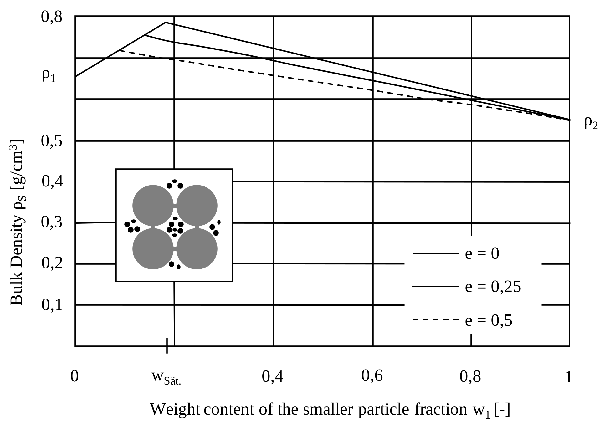
For both polymer blends and filled systems (compounds), the granule diameter of the smaller fraction is assumed to be much smaller than that of the larger fraction ($d_1 \ll d_2$). If the bulk density $ρ_{S.MIX}$ of a mixture composed of two different particle fractions is plotted against the weight fraction of the smaller fraction $w_1$, each curve exhibits a maximum at the saturation concentration $w_1 = w_{Sät}$, independent of the void fraction $e$. The saturation concentration is calculated as:
$$w_{Sät} = \frac {ρ_2 \cdot (1-p_∞) \cdot (1-e)}{ρ_1 + ρ_2 \cdot (1-p_∞) \cdot (1-e)}$$
with the maximum packing fraction for a cubic-close-packed arrangement of spheres:
$$p_∞ = \frac {V_{sphere}}{V_{total}} = \frac {π}{3 \cdot √2} ≈ 0,74$$
Here, $V_{sphere}$ is the volume that the larger material component (Mat. 2) can maximally occupy relative to the total volume $V_{total}$. The void fraction that is too small for the smaller component (Mat. 1) to fit is set to $e = 0.25$. From this, the saturation bulk density (bulk density of the mixed region) is obtained:
$$ρ_{Sät} = ρ_1 + (1-ρ_∞) \cdot (1-e) \cdot ρ_2$$
To determine the bulk density $ρ_{S.MIX}$ of multicomponent systems in polymer blends and compounds with $d_1 < d_2$, three cases are distinguished. The procedure for the three calculation types is illustrated in the following figure. The subdivision criterion in all calculation types is the ratio of the particle diameters ($d_1 / d_2$). Initially, only two calculation approaches are used ($d_1 < 0.25 \cdot d_2$ or $d_1 > 0.75 \cdot d_2$), while the third calculation approach is obtained by linear averaging of the other two in the transition range ($0.25 \cdot d_2 < d_1 < 0.75 \cdot d_2$).
Bulk Density of Multicomponent Systems (Polymer Blends and Compounds with $d_1 < d_2$)
Calculation Type I (if $d_1 \ll d_2$, i.e., $d_1 < 0.25 \cdot d_2$)
- if $w_1 < w_{Sät}$
$$\rho_{Mix} = \left(1 - \frac{w_1}{w_{Sät}}\right)\rho_1 + \frac{w_1}{w_{Sät}} \rho_{Sät}$$
- if $w_1 \geq w_{Sät}$
$$\rho_{Mix} = \left(1 - \frac{1 - w_1}{1 - w_{Sät}}\right)\rho_2 + \frac{1 - w_1}{1 - w_{Sät}} \rho_{Sät}$$
Calculation Type II (if $d_1 > 0.75 \cdot d_2$)
$$\frac{1}{\rho_{Mix}} = \frac{w_1}{\rho_1} + \frac{w_2}{\rho_2}$$
Calculation Type III (if $0.25 \cdot d_2 < d_1 < 0.75 \cdot d_2$)
$$\rho_{Mix} = \frac{(\rho_{Mix I} + \rho_{Mix II})}{2}$$
Here, $\rho_{Mix}$ is obtained by linear averaging of Calculation Types I and II.